Sign-Lingual: From Pixels to Predictions 👐
At the start of the year, I was on a train heading back home from London. As is often the case with many train journeys in the UK, there was a route disruption that led to the destination being a few stops earlier than originally planned.
During the disruption, I noticed a passenger who was hard of hearing struggling to understand the onboard announcements. In that moment, I realised the challenges that people with hearing impairments still face today, despite all the technological advancements we’ve made. It was then that I thought:
What if there was an app that could help signers and non-signers communicate more easily?
As part of the BrainStation bootcamp I attended, each student was tasked with creating a real-world project that could be solved using machine learning methods. I saw this as a perfect opportunity to develop a tool that could make a meaningful impact, introducing: Sign-Lingual.
Sign-Lingual is a sign language recognition tool designed to translate American Sign Language (ASL) using deep learning techniques.
Defining project scope
At first, it was overwhelming to consider all the potential directions for this project. I initially struggled with where to start. To tackle the task, I found it helpful to first envision the model’s core functionality. The ideal app would facilitate two-way communication: from signer to non-signer and vice versa.
For simplicity, I decided to focus on the first communication path: enabling signers to communicate with non-signers. This approach allowed me to create a rough mock-up of what I wanted to build.
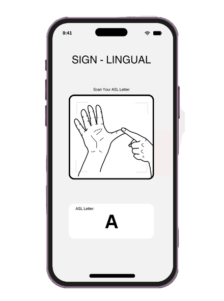
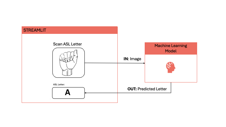
The core functionality of the app involves capturing a real-time image of an ASL letter. The app then uses a machine learning model to return a prediction of that ASL letter. Of course, there’s a lot more happening behind the scenes so let’s dive into the details!
Data Overview
To begin my project, I chose to work with the MNIST Sign Language dataset, available via openML. This dataset was ideal for multiple reasons: the images are well centered, feature a clear background and have minimal augmentation making it a suitable benchmark to start with. Each letter in the dataset has approximately 1400 images, providing a solid foundation for training. However, it’s important to note that the dataset does not include data for the letters ‘J’ and ‘Z’ since these letters involve moving parts, which static images in the dataset cannot capture. Its simplicity made it a good starting point for me especially since this was my first image recognition project.
As the project progressed, I expanded my dataset to include some real-life, coloured images captured using Teachable Machine. For each letter, there are 600 images. As like the MNIST dataset, there is no data for letters ‘J’ and ‘Z’. The purpose of this addition was to enhance the model’s ability to generalise to images with various augmentations.
Data Preparation
As with any data science project, preparing the data is a crucial step before modelling can begin. The same applies for image data. Image data processing involves some unique techniques compared to traditional data.
Note: Below are all the different types of data preparation I carried out, bear in mind not all models required all these steps to be taken.
Resizing/Reshaping
The MNIST dataset consists of 28x28 pixel images, totalling 784 pixels per image.
For real-world images captured using Teachable Machine, the images were reshaped to 64x64 pixels. This higher resolution allows for more detail and context, which can improve the model’s performance. However, this comes with a trade-off: increased computational requirements. As a result, expanding the resolution beyond 64x64 pixels was not feasible, as the training time for the transfer learning models increased exponentially.
Scaling
Pixel values range from 0 (black) to 255 (white), scaling pixels to a range of 0 to 1 ensures all features (pixels) contribute evenly to the model’s training. This leads to an improvement in the model’s performance and prevents any biases towards the larger pixel values.
In neural networks, scaling is also important due to the activation functions which perform better when input values are within a normalised range. Proper scaling allows the network to be more consistent and balanced when updating the weights during training.
Data Augmentation
Data augmentation describes the process of adding ‘noise’ into your data to simulate conditions faced in the real-world. For image data, this process includes techniques such as rotating, flipping and cropping images. These transformations help create a more diverse set of training data, making the model more robust and capable of generalising to new, unseen images.
In this project, data augmentation was applied to the training set only. By doing so, the model was exposed to a variety of image augmentation during training in attempt to improve its ability to handle different scenarios in the real world. The validation set images were not augmented, allowing us to evaluate the model’s performance on unaltered images. This ensures that the model’s ability to generalise to real-world data is assessed rather than its ability to cope with artificially created noise in images.
To implement data augmentation, I used Keras, a deep learning library. Keras has an ImageDataGenerator class which performs augmentation in real time. Given a set of images, the class will apply random transformations on the images.
Note: Only a randomly selected subset of images undergo augmentation, this is controlled by the parameters the user enters. This ensures variation is introduced into the dataset without over confusing the model during training.
Example:
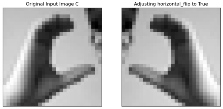
Flipped the image horizontally, this augmentation technique is particularly useful in sign language as it accounts for signs with either the left or right hand.
Here is a list of augmentation I applied using ImageDataGenerator:
| Augmentation Applied | Value | Explanation |
|---|---|---|
| rescale | 1/255 | Normalisation of the input data |
| rotation_range | 20 | Ensures model can deal with slight tilts in the hand position, most likley to occur in the real world |
| width_shift_range | 0.1 | ensure model can deal with off-centered images |
| height_shift_range | 0.1 | To ensure model can deal with off-centered images |
| shear_range. | 0.2 | To distort the image, like when we see objects from different perspectives |
| zoom_range. | 0.2 | Zooms in and out of images so model can recognise signs when hands are of different sizes/further/closer. |
| horizontal_flip | True | To mimic opposite hand, if original image is left hand, we can flip the image to show right hand |
Feature Extraction with HOG and LBP
Feature extraction describes the process of manually extracting meaningful features from raw image data to transform it into a more compact, reduced set of features. This process simplifies data by reducing its dimensionality while preserving only the important parts of the images.
For the Sign-Lingual project, I applied the following feature extraction methods:
HOG (Histogram Oriented Gradients)
- Identifies edges and textures from raw input image data by comparing gradient changes between pixels in images.
- Captures overall shape and structure of hands.
LBP (Local Binary Patterns)
- Identifies textures from raw input image data by comparing each pixel with its neighbouring pixels.
- Detects patterns and textures of hands.
Colour Histogram
- Shows the distribution of colours within an image.
- Helps to identify and differentiate between signs based on colour variations.
After applying these methods, each image is now represented as a feature vector, where different parts of the vector come from each extraction method above. By representing images as feature vectors, the model can focus on specific patterns and details during training. This manual extraction process helps the model to better identify subtle differences that might be overlooked when using raw pixel data alone, leading to improved performance and accuracy in predictions.
Data Splitting
Data splitting involves separating the dataset into subsets to ensure effective model training and evaluation. For my project, I split data into three subsets:
1. Training Set
- Used to train models, this in includes 80% of the total data.
- With this data, models lean patterns and relationships for each different sign.
2. Validation Set
- The remaining 20% of the data.
- Used to evaluate model performance, gives an indication how well the model generalises to unseen images.
3. Test Set
- The test set were a portion of the real-world images I captured using Teachable Machine.
- Used to do final model evaluations testing each model’s ability to classify real-world images.
Modelling Approach
In this project, I explored a series of modelling techniques commonly used for image recognition starting with simpler methods and progressing towards more complex approaches. This helped me to understand the fundamentals concepts of image processing as well as how advanced models can be used to improve model performance.
In this section, I will outline the different approaches:
Baseline Logistic Regression
The initial approach involved logistic regression where each pixel represented a single independent feature. For a greyscale image of 28 by 28 pixels, there are 784 independent features. Each feature corresponds to a single pixel’s intensity.
We can think of the problem as a simple classification task. The model ‘learns’ particular arrangements of differing pixel intensities for each letter. When performing classification, the model inspects the given image to identify specific arrangements and make a letter prediction.
So, what exactly is the model learning?
To uncover what the model is learning for each letter, I created a function that plots the mean image of a given letter next to the letter’s odds ratio. This allows us to gain an understanding into the model’s classification process and provides an insight into what is happening behind the scenes.
Let’s look at letter A as an example:
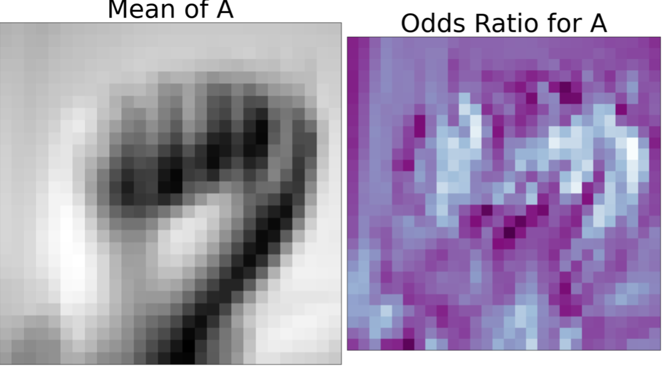
The darker areas in the right image highlight areas of significance for letter A. These areas correspond to higher odds ratios, meaning the pixel intensities in these areas are the mode defining for classifying a letter as A. Looking at the image on the left, we can see that the darker areas correspond to the curling of the fingers, the opening of the palm and edges of the closed fist – all of which are key features the model uses to classify an image as letter A.
Results
The results table below compares the performance of the baseline logistic regression model with and without data augmentation. As mentioned earlier, data augmentation of images was used to introduce some variability into the dataset and to assess how well the model handles noise.
| Without Data Augmentation | With Data Augmentation | |
|---|---|---|
| Train Score | 99.99 | 31.72 |
| Validation Score | 99.99 | 25.82 |
Without data augmentation, the model performs very well on both the training data and validation data. Given the near-perfect scores, why should we progress to exploring different models?
The reasoning becomes clear when we look at the model’s performance with augmented data. Both the training and validation scores drop significantly suggesting the logistic regression model struggled to identify distinguishing features for each letter when the data contained more noise.
The difference in results emphasises the limitations of the baseline model. Logistic regression struggles in handling difficulties data augmentation introduces, a model which only assesses raw pixel values is too simple. In real-world scenarios, this model would fail to adapt to inevitable noise.
To address these limitations, the next step involves using feature extraction methods. Unlike raw pixel values, which can be highly sensitive to noise, feature extraction methods focus on extracting more meaningful features such as edges and textures from the images. By providing the model with more meaningful features, it becomes better at handling noise.
Logistic Regression with Feature Extraction
After discussing the limitations of using raw pixel data in logistic regression, the next step was to enhance the model’s performance using feature extraction methods discussed earlier. Instead of training the logistic regression model on a flattened array of raw pixel values, the model is now trained on feature vectors.
Results
The tables below compare the performance of the baseline logistic regression to the logistic regression model with feature extraction for both non-augmented and augmented data.
Without data augmentation:
| Logistic Regression Model | Logistic Regression Model with Feature Extraction | |
|---|---|---|
| Train Score | 99.99 | 99.03 |
| Validation Score | 99.99 | 98.86 |
With data augmentation:
| Logistic Regression Model | Logistic Regression Model with Feature Extraction | |
|---|---|---|
| Train Score | 31.72 | 48.11 |
| Validation Score | 25.82 | 58.60 |
It is clear the introduction of feature extraction significantly improves the model’s ability to generalise.
Performance of the model with feature extraction on non-augmented data remains high. This suggests that the feature extraction methods effectively capture the key features of the images, allowing the model to maintain accuracy despite the reduction in data dimensionality.
The real advantage of feature extraction is seen in the model’s performance with augmented data. The model with feature extraction outperforms the baseline model, demonstrating its improved ability to cope with noise by helping the model better differentiate between important features and irrelevant noise. This makes the model less susceptible to noise introduced by data augmentation improving its performance.
While feature extraction offers benefits to model performance, we must extract features manually and this requires some knowledge to do this correctly. Again, it is possible that some patterns are overlooked and missed. To address this, it would be best to use automated methods such as deep learning techniques, where relevant features are learnt directly from the data. The next step was to explore Convolutional Neural Networks (CNNs) and how they automatically learn and extract features from images.
Convolutional Neural Networks (CNN)
CNNs are a type of neural network designed specifically for image/video processing. CNNs mimic the way we as humans process image data as they too can recognise patterns and shapes in images. Unlike traditional neural networks, CNNs include convolutional layers that detect features such as shapes and edges, enabling automatic feature extraction from raw data.
How do CNNs recognises shapes/objects in images?
Let’s start with an example.
Imagine a house:

We as humans see a house and can identify features of the house such as windows, a door, a roof and a chimney.

If we break down these features, all the listed objects are made up of the following lines:

CNNs follow a similar process but in reverse. Instead of starting with a complete object (a house), CNNs begin by detecting basic elements such as lines and edges. These elements form more complex shapes like the windows and roof. Through the layers of the network, these simple elements combine to produce more complex shapes and eventually the network progresses and learns enough to identify the full object like the house.
CNN Architecture
Brief outline of the CNN I built for my project:
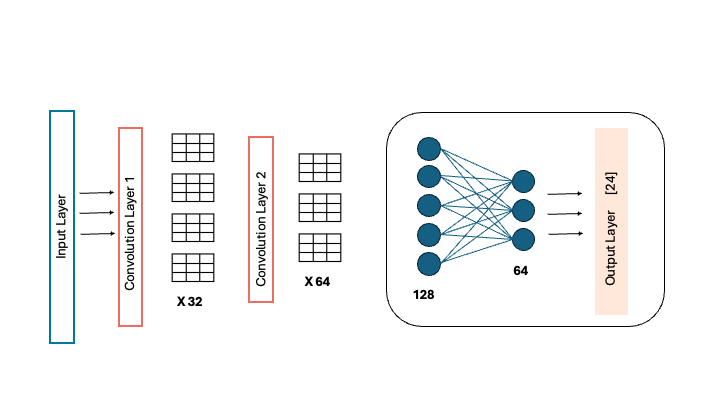
Since the MNIST dataset I was working with is relatively small compared to typical image datasets, I decided on a simple convolutional neural network (CNN) with six layers. The structure of the network is as follows:
1. Input Layer: This layer receives the images as input.
2. Convolutional Layer 1: The first convolutional layer applies filters to detect basic features such as edges.
3. Convolutional Layer 2: The second convolutional layer builds on the features detected by the first layer, recognising more complex patterns and shapes.
4. Fully Connected Layer 1: This layer begins to combine the detected features from convolutional layers to gain an understanding of the overall image.
5. Fully Connected Layer 2: Building on the output of first fully connected layer, fine-tuning it before classification.
6. Output Layer: The final layer outputs the model’s predictions, classifying the input image as a single letter.
Filters/Kernels
Filters, also referred to as kernels, are typically a 3 by 3 grid of weights used by CNNs convolutional layers to detect features in the input image. These weights are initially set randomly and are adjusted during the learning process through backpropagation to minimise the model’s loss. Each image detects a particular feature with the first few filters detecting simple features like edges. The deeper we go into the network the more complex these features will be.
How filters work:
Each filter slides over the input image, this process is called convolution. At each position, the filter’s weights are multiplied with the pixels of the image, the results of the multiplications are added to produce a single value for that position.
The result of a filter convolving across an image is called a feature map. Each filter produces its own feature map where specific features of that filter are highlighted. The feature map of the first convolution layer is passed as input to the second, this allows the network to learn increasingly complex features as it gets deeper.
In my CNN, the first convolutional layer contains 32 filters each detecting simple features. The second convolutional layer contains 64 filters, these filters detect more complex features building on the output of the first convolutional layer.
Inspecting CNN’s layers
To gain deeper insights into kernels and feature maps, I created a function to visualise the kernels and their outputs for a given convolution layer. This function provides insight into how kernels extract and highlight features from specific letters in the MNIST dataset.
Convolution Layer 1 Output – Kernel 13

By looking at the weights of kernel 13, we can gain valuable insights into the features it detects. Darker regions signify larger weights suggesting these regions represent patterns which the filter is searching for in the input image. This kernel has identified patterns related to the curled fingers of the hand and edges, suggesting that it plays a crucial role in distinguishing between open and closed hand signs.
Convolution Layer 2 Output – Kernel 2

Here we can see the second layer kernels are harder to interpret when compared to the input image. The reason for this is that these kernels are applied to the output of the previous convolution layer. Kernels in the second layer have learnt to detect more abstract patterns often from combining the output of the previous convolutional layer. The deeper the convolutional layers get, the more abstract and complex the features become making it more challenging in terms of interpretability.
Results
| CNN | CNN with augmentation | |
|---|---|---|
| Train Score | 99.30 | 79.89 |
| Validation Score | 99.26 | 92.78 |
Base CNN Model:
The base CNN model achieved high results, with a training accuracy of 99.30% and a validation accuracy of 99.26%.
These scores indicate that the model effectively learned from the MNIST sign language dataset and demonstrated strong ability to generalise as seen by the minimal difference between training and validation scores.
CNN Model with Augmentation:
Accuracy scores show a reduced performance compared to the base CNN model, with training accuracy dropping to 79.89% and validation accuracy at 92.78%.
The drop in training accuracy suggests that augmentation introduced variability that the model struggled to manage, causing some confusion during training. However, the high validation score indicates that the model became better at generalising to new, unseen variations of the data.
CNN works by learning features from a given dataset and then uses these features to classify images. While this has proved to be the most effective method so far in terms of performance with augmented and non-augmented data, it would be interesting to assess the performance of pre-trained models. Pre-trained models are trained on very large and diverse image datasets. We can leverage features the model has already learnt and fine tune the model for sign-language recognition. Since pre-trained models have encountered a broad range of images during their initial training, they are better equipped to handle variations in data making them more robust.
Transfer Learning
Transfer learning is a technique in machine learning where a pre-trained model is adapted and fine-tuned to a complete a given task. Instead of training a model from scratch, transfer learning leverages knowledge the pre-trained model has from its initial training and applies it to a specific task.
For this project, I explore two pre-trained models: ResNet-50 and VGG-16 using Keras. Both are pre-trained on ImageNet, a dataset consisting of millions of images across thousands of different categories.
The input image dimensions for these models were 64 by 64 pixels and included all three-color channels (RGB). Pre-trained models are designed to interpret colour and have likely learned features based on colours, so using grayscale images would not leverage these learned features. In addition, I increased the image resolution from 28x28 to 64x64 pixels to maintain the integrity of images. Pre-trained models are quite deep and have multiple layers, higher resolution images ensure effective learning with minimal information loss.
The process of transfer learning for both models was the same:
1. MNIST Dataset: The first stage involved fine-tuning the pre-trained models using the MNIST dataset. This initial fine-tuning adapts the model to recognise patterns relevant to this specific dataset.
2. Augmented Dataset: Fine-tuning was performed using the augmented images from the MNIST dataset. This step helps the models adapt to variations introduced through data augmentation, such as rotations and distortions.
3. Teachable Machine Images: Top-up training using images captured from Teachable Machine. In this process, I froze all layers apart from last few fully connected layers, training only these layers. The purpose of this was to refine the models on images with real-world variations that are not present in the MNIST data.
ResNet-50
ResNet-50 is a deep CNN with 50 layers. ResNet-50 utilises residual blocks and skip connections both of which allow the model to be 50 layers deep while still maintaining high performance - I will provide further detail on how residual blocks work in a future post.
Results
| ResNet | ResNet with augmentation | ResNet Top Up Trained | |
|---|---|---|---|
| Train Score | 99.99 | 89.27 | 70.60 |
| Validation Score | 99.88 | 98.28 | 68.53 |
Initially, the ResNet-50 model scored high accuracy with a training score of 99.99% and a validation score of 99.88% when trained on the original MNIST dataset. However, when augmented data was introduced, the performance decreased, with training and validation scores dropping to 89.27% and 98.28%, respectively. This indicates that while ResNet-50 is effective in handling the original dataset, it struggled a little with the noise introduced by data augmentation.
The most significant drop in performance occurred during top-up training with images from Teachable Machine, where the training score fell to 70.60% and the validation score to 68.53%. This suggests that the model’s ability to adapt to real-world variations was limited, likely due to the relatively small size of the dataset – only ~600 images per class. This dataset size may not provide enough data for the deeper layers of ResNet-50 to effectively learn which impacts the model’s performance.
VGG-16
VGG-16 is a deep convolutional neural network with 16 layers: 13 convolutional layers and 3 fully connected layers. It uses a block-based structure where each block includes several convolutional layers followed by max pooling. This design helps the network maintain its depth while preserving image dimensions, enhancing feature extraction and overall performance.
Results
| VGG Model | VGG with Augmented Data | VGG Top Up Trained | |
|---|---|---|---|
| Train Score | 99.98 | 93.70 | 99.68 |
| Validation Score | 99.83 | 98.98 | 99.49 |
The VGG model performed well, with a training score of 99.98% and a validation score of 99.83% when trained on the original MNIST dataset. Introducing augmented data led to a decrease in the training score to 93.70%, though the validation score improved to 98.98%. This indicates that while the VGG model adapted well to the augmented data.
Top-up training with additional data did not improve on the training or validation score suggesting the dataset may have been too small.
It looks like VGG has outperformed all other models in its ability to classify images, deal with augmented data and real-world images. With a larger and more diverse dataset, it is possible that the ResNet-50 model could perform better than VGG-16. This is an area worth exploring in the future as increasing the dataset size might allow ResNet-50 to leverage its deeper architecture and residual blocks more effectively.
Model Selection and Deployment
So far, from all the models we have explored, the VGG-16 model stands out as the most effective for real-time prediction. Its robust performance in handling augmented and real-world images makes it the ideal choice for deployment.
To productionise the VGG-16 model, I used Streamlit - a tool for creating interactive web apps.
How to productise a model using Streamlit
Firstly, I saved the VGG-16 model after top-up training as a .h5 file, which is the recommended format for Keras models.
After exploring Streamlit’s documentation, I discovered that it supports camera input, allowing for real-time image capture. This feature enables users to take images and feeds them directly into the model for predictions.
The next step was to reformat the captured images to match the input dimensions required by my model—64 pixels by 64 pixels with three colour channels. This is where I encountered an issue as the camera input in Streamlit was rectangular and my model was expecting square images.
Initially, I used TensorFlow’s tf.image.resize function to adjust the image dimensions. However, this approach either stretched the image or added black padding when I set the preserve aspect ratio parameter to True.
To resolve this, I needed to crop the image before resizing it. After several attempts and failing to find a suitable TensorFlow function, I manually calculated the aspect ratio to perform cropping and resizing separately. Although this solution worked, it introduced a new issue: if the user was not positioned correctly in the frame, the cropped image may not capture their full hand. To address this, I printed a preview of the cropped image to ensure the user is in frame.
Mini Demo
What’s next?
Looking ahead, there are several improvements I could make to this project.
One key area of focus is refining the deploymeny of my model. Currently, I am using Streamlit to deploy a web app for real-time image capture and prediction. While this approach works well, it requires users to have the python file downloaded and access to the trained VGG-16 model. To make the app more accessible, I should look into using APIs to deploy my model. Using something like Fast API allows users to interact with the model without needing to download or manage code themselves.
Another development I can make is to predict complete words instead of predicting individual letters. To make this a possibility, requires implementing a continuous image capture loop. I will investigate if this can be done using OpenCV library.
Additionally, reaching out to sign language communities and experts would be a useful step for further development. Engaging with signers will provide valuable insights into common misunderstandings allowing me to assess if the model replicates these issues. This feedback will guide fine-tuning and adjustments to improve the model’s accuracy.
Finally, addressing the issue of backgrounds in images is another important step. Currently, the model’s performance can be affected by varying backgrounds. To deal with this, I plan to investigate methods for background removal using OpenCV before images are fed into the model.