Trick Or ReTreat: Building a Custom Environment - Phase 3 🚪
In the previous phase of my custom environment, I added in candies and ghosts which acted as rewards and penalties. Using Q-learning, I trained the agent to navigate through the updated environment. After testing the agent and inspecting the Q-table, it was clear that the agent successfully learned to complete the task.
For the next phase, Phase 3, I am taking the environment one step further by randomising the initial positions of the ghosts in the grid at the start of each episode. This increases the state space drastically making Q-learning inefficient. To tackle this, I plan to use Deep Q-Networks (DQN), which are better suited for environments with larger state spaces.
Let’s first see what has changed in the environment!
Environment Updates
As stated above the final environment now includes setting the ghosts to random positions at the start of each episode. The agents objective is the same: to reach the door while avoiding the ghosts and collecting as many candies as possible.
Like in the previous post, I will only be including code snippets of methods I have changed. To see full class with all methods, please visit the my GitHub repository.
1) init: Initialises Environment

-
Removed the static positions of ghosts and set all ghosts to be out of bounds.
-
The positions of each ghost will be set randomly in the
resetmethod.
2) reset: Resets the Environment to an Initial State
-
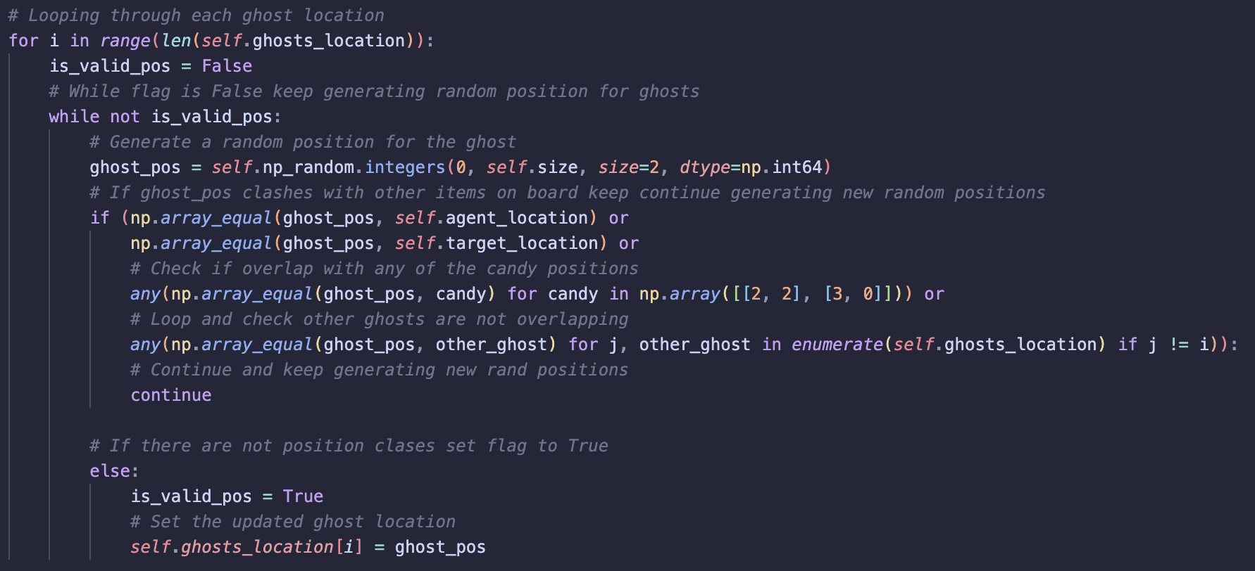
In the reset, I am already setting the agent to a random position on the grid, I use the same method to randomise the initial positions of each ghost.
-
Added constraints (explained below) to avoid confusing the agent with rewards and penalties in the same cell.
3) step: Agent takes action
-
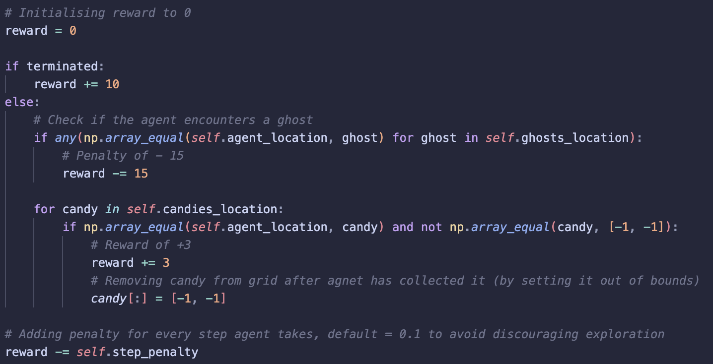
I fine-tuned the reward structure for better performance using a trial-and-error approach.
-
The rewards/penalties are less drastic compared to those used in Q-learning. I assume this is as DQNs are more advanced and allow for greater exploration without the agent getting stuck – something I saw when fine-tuning rewards for Q-learning.
Deep Q-Networks
What is DQN?
DQN is a reinforcement learning method that combines Q-learning with deep learning (neural networks) to find optimal Q-values for each action in the action space. Just like in Q-learning, the agent uses these Q-values to select action with the highest estimated reward.
In Q-learning, a Q-table is used to store Q-values for each state-action pair and these values are updated by the agent as it interacts with the environment. This approach is best suited to environments with small state spaces like seen in Phase 2 of my custom environment. As the state space grows, the Q-table also grows and becomes too large.
DQN addresses this state space problem since it uses a neural network instead of a Q-table. The network takes in an environment state as an input and outputs Q-values for all possible actions. However, despite these differences, DQN still uses part of the Q-learning formula to update its Q-values. DQN also makes use of experience replay and target networks to stabilise the agents learning – I explore these further below.
This is what a simple overview of what a DQN may look like:
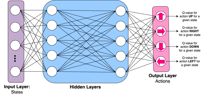
Input Layer: Each node represents an environment state.
Hidden Layer/s: Where the learning occurs, using weights and biases the network starts to learn which actions are most rewarding for a given environment state.
Output Layer: Each node represents an action from the action space, in my project there are 4.
Why DQN?
Initially, with only the agent moving, the state space was only 25. By randomising the ghosts’ initial position in the environment, the state space has grown, approaching 200,000 possible states. Here’s how:
-
The agent can occupy any of the 25 cells on the grid, resulting in 25 possible positions.
-
Each ghost is slightly more restricted in its placement:
-
Ghost 1: Has 21 valid positions, as it cannot overlap with the agent, the target (door), or the two candies.
-
Ghost 2: Has 20 valid positions, as it cannot overlap with the agent, the door, the two candies, or Ghost 1.
-
Ghost 3: Has 19 valid positions, as it cannot overlap with the agent, the door, the two candies, Ghost 1, or Ghost 2.
-
I added in these constraints to ensure that cells don’t offer rewards (candies) and penalties (ghosts) at the same time as this could confuse the agent.
-
The total number of valid positions for the ghosts is:
-
Total State Space (including the agent) is:
\[7980 \times 25 = 199,500\]
How DQNs work?
So far, I have explained how DQN builds on Q-learning by using a neural network instead of a Q-table to estimate Q-values. But how do DQNs actually work?
First let’s take a look at the main concepts:
Experience Replay
-
Experience Replay allows the agent to train on past experiences by storing each interaction the agent has with the environment in a Replay Buffer.
-
Each interaction with the environment is stored as a tuple:
(current state, action taken, reward, next state)
-
The Replay Buffer has a fixed size (parameter to be set by the user), training only begins once enough experiences are stored.
Policy Network
-
The Policy Network is the main network the agent uses to select actions and learn.
-
Input: The current state of the environment.
-
Output: Q-values for all actions in action space.
Target Network
-
The Target Network is a copy of the Policy Network, it has the same architecture.
-
The purpose of the Target Network is to tune the weights of the Policy Network.
-
It calculates target Q-values using the Bellman equation:
- The target Q-value represents the estimated optimal future reward the agent can achieve from a given state-action pair.
Backpropagation
- The loss between the Q-values predicted by the Policy Network and the target Q-values is calculated:
- This loss is then backpropagated through the Policy Network to adjust the weights.
Note: The target network’s weights stay fixed during backpropagation and are periodically updated from the policy network. This ensures the policy network has a stable point of reference during training.
Goal of DQN
-
The agent is trying to learn a policy that maximises the future long-term reward, like in Q-learning.
-
The Q-values predict the future reward for each state-action pair.
-
The goal is for the policy network to accurately predict Q-values to maximise the future rewards.
Diagram
This is an overview of how I understand DQNs work:
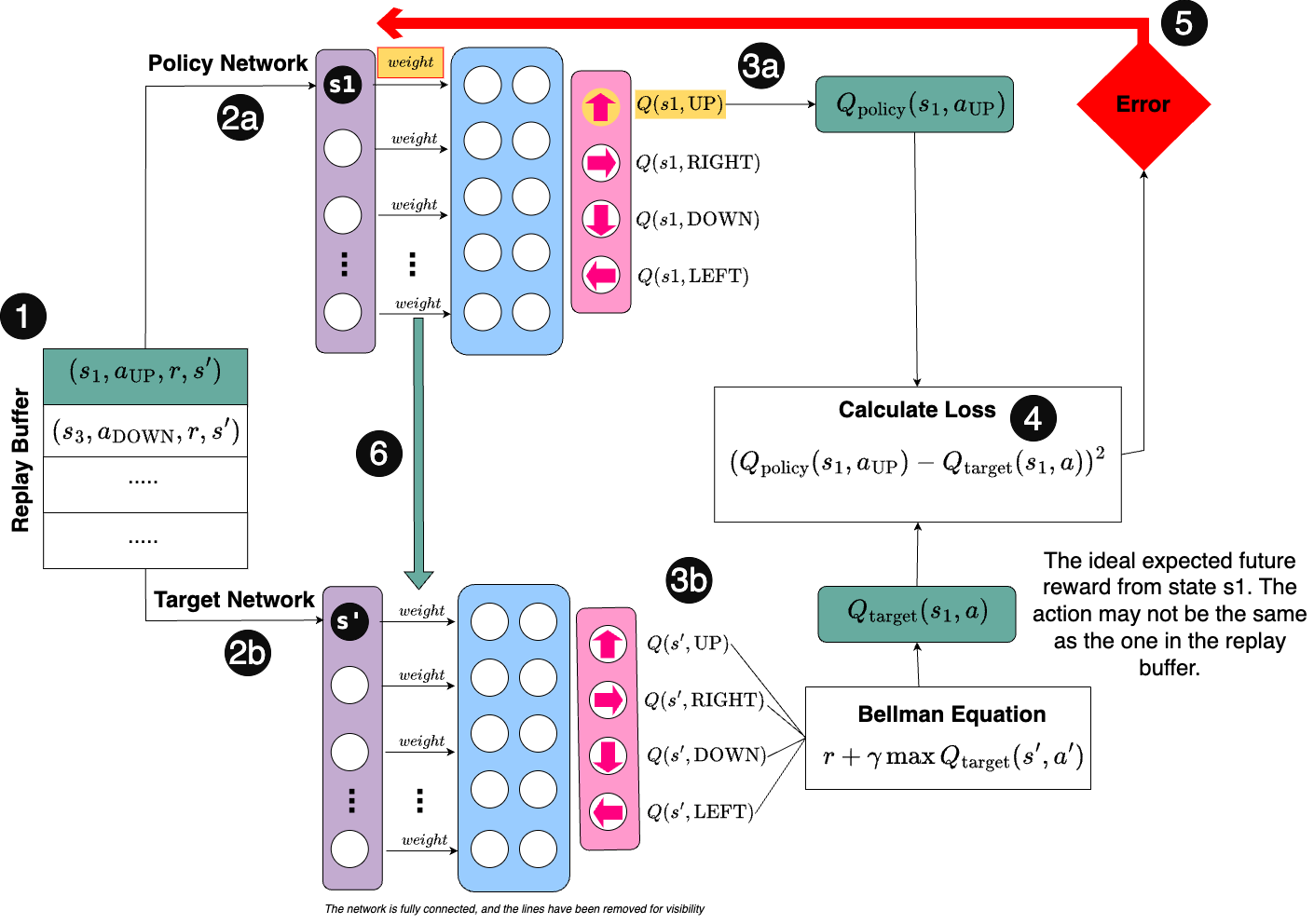
Both networks are fully connected - the lines have been removed for visibility.
There is a lot going on, so let’s break it down step by step!
Step 1
Random batches of experiences are sampled from the Replay Buffer. This is to ensure the agent doesn’t just focus on short-term patterns and learns more generalised, long-term patterns.
Step 2a
The current state (s1) from the Replay Buffer is passed through the Policy Network. The network uses its hidden layers to output Q-values for each possible action in that state.
Step 2b
The next state (s’) from the Replay Buffer is passed through the Target Network, which outputs Q-values for each possible action in the next state.
Step 3a
From the Policy Network, we focus on the Q-value corresponding to the action the agent took in state s1 (from the replay buffer).
For example, if the action was UP, we look at the Q-value for UP from s1.
Step 3b
Using the Bellman equation, we calculate the target Q-value.
\[Q(s, a) = r + \gamma \max Q(s', a')\]This represents the maximum possible future reward the agent could achieve if it follows the optimal policy.
This target Q-value represents the ideal future reward the agent would get if it followed the optimal policy (considering immediate and future rewards). The Policy Networks predictions should be as close to this value as possible.
Step 4
The loss is calculated as the difference between the predicted Q-value from the Policy Network and the target Q-value.
\[\text{Loss} = (Q_{\text{policy}}(s, a) - Q_{\text{target}}(s, a))^2\]Step 5
The error (loss) is backpropagated through the policy network and the weights of the Policy Network are updated to reduce the loss and improve Q-value predictions.
Step 6
Periodically, after a set number of steps (also a parameter), the weights from the Policy Network are copied over to the Target Network. This prevents the Target Network from changing too quickly and helps to stabilise learning.
Implementing DQN
To implement Deep Q-Networks for my environment, I decided to use the Stable Baselines 3 library. Initially, I attempted to build my own DQN from scratch. Despite understanding the basics of DQNs, I was still unable to get my own to work. Given I have already spent a lot of time on this project, I decided it best to move on and use the Stable Baselines 3 library instead.
If you’re interested in seeing my attempt to build the DQN from scratch, I’ve included it in the Appendix of the final environment notebook.
Step 1: Create a vectorised environment

The first step in implementing DQN was to create my environment and then vectorise it using the DummyVecEnv wrapper from Stable Baselines 3. In this phase, I decided to use 5 instances of my environment, allowing the agent to be trained on all 5 environments at the same time.
The step penalty requires careful balancing, so I decided to set it to –0.6 for DQN. This choice was based on the following considerations:
-
Not too harsh: To allow for necessary exploration and prevent the agent from settling on suboptimal paths.
-
Not too lenient: To discourage wandering and ensure the agent focuses on efficient paths toward the target.

I then wrapped my vectorised environment using VecMonitor instead of Monitor since I have multiple environments. This wrapper allows access to the training logs of my agent, which I will share and analyse later in this post.
Step 2: Define the DQN model

I called DQN from Stable Baselines library and set my paramters:
policy:MultiInputPolicy
Setting the policy model to MultiInputPolicy since observations are stored as a dict.
env:learn_env
The environment the agent interacts with and learns from.
buffer_size:150,000
Controls size of the replay buffer, I chose 150,000 to capture a diverse range in the agent’s previous experiences so the agent can learn more generalised patterns.
batch_size:256
Batch size refers to the number of experiences the agent samples from the replay buffer to update the weights in the policy network. I set this to 256 as using a larger batch helps ensure more stable and reliable updates.
learning_rate:0.0005
Learning rate controls how fast the agent learns, I set this to 0.0005 as I wanted updates to be made to the Policy Network to be small in order to smooth learning with stable weight updates.
target_update_interval:10,000
Updates the Target Network with the weights of the Policy Network every 10,000 steps.
exploration_final_eps:0.05
Final value of epsilon after it has decayed, I set this to 0.05 so 5% of the time the agent will explore by taking new actions. I thought this would be good and would make the agent more adaptable in an environment where penalties are randomly placed.
exploration_fraction:0.8
Controls the amount of steps epsilon decays over, 0.8 means epsilon decays over 80%. 80% of the training is where the agent is exploring, the remaining 20% the agent focuses on exploitation. I thought this best due to the randomness of the ghosts, a higher exploration could help the agent adapt better.
To see the DQN network architecture, visit the final_environment notebook.
Step 3: Train the agent and save the model

Use .learn to train the agent and save the model for easy access if needed in the future
Evaluation of Training
From extracting the logs, I can look at the rewards and lengths of the episodes during training. This allows me to assess the learning process.
Rewards Across Training
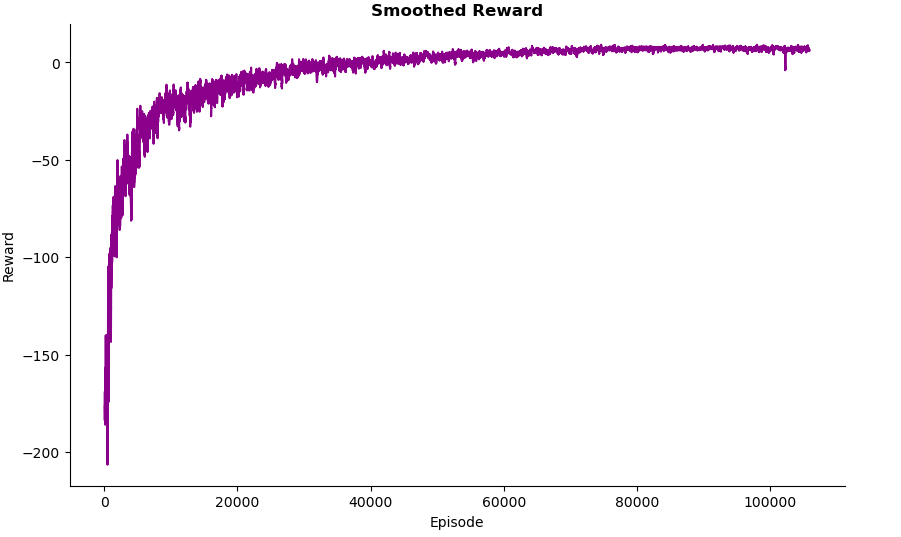
Early in the training, the rewards vary a lot. This makes sense as this is when the agent is exploring the environment, taking random actions. As the episodes progress, rewards increase - this shows the decay of epsilon as the agent starts to explore less.
After 40,000 episodes, the curve flattens, and the rewards start to stabilise. This is a sign the agent has successfully learned the task well and its performance is now stable. After 50,000 episodes, the agent’s performance no longer improves much suggesting the agent has reached a near optimal policy.
Overall training the agent aligned with typical patterns seen from RL agents. The agent gradually shifts from exploration to exploitation with the learning curve flattening as it reaches a near-optimal policy.
One noticeable difference between DQN training and Q-learning training is that DQN’s train over a larger number of episodes. This is likely due to how DQNs train using neural networks, networks require a lot of data to train and learn effectively.
Testing
Visualisation
Results
| Episode | Score |
|---|---|
| 1 | 10.0 |
| 2 | 11.2 |
| 3 | -5.6 |
| 4 | 8.2 |
| 5 | 10.0 |
| 6 | 10.6 |
| 7 | 10.6 |
| 8 | 10.0 |
| 9 | 10.6 |
| 10 | -5.0 |
| 11 | 10.0 |
| 12 | 10.0 |
| 13 | 10.0 |
| 14 | 10.0 |
| 15 | 11.2 |
| 16 | 9.4 |
| 17 | 10.0 |
| 18 | 11.2 |
| 19 | 9.4 |
| 20 | 10.6 |
High Scores (9.4 and above):
-
The agent performs consistently well in most episodes, showing it effectively avoids ghosts and maximises rewards.
-
High scores indicate that the agent has learned to prioritise reaching the door and if sensible, collects candies along the way.
Poor Performance (Episode 3 and 10):
-
In Episodes 3 and 10, the agent encountered a ghost on the way to the door. This might be due to the remaining 5% exploration rate, causing the agent to take random actions occasionally and follow suboptimal paths.
-
Could also be the total rewards gathered during the episodes outweighs the penalty of a ghost.
-
Potentially worth exploring with ghost penalties in the future, but also must be cautious not to increase too much as this may cause the agent to become stuck.
Overall, the scores reflect a strong understanding of the environment, with a few lapses in performance.
Summary
In the final phase of this project, I extended my custom environment by randomising the starting positions of the three ghosts. This change caused a state space explosion, making the Q-Table too difficult to use. To address this, I trained my agent using Deep Q-Networks (DQNs), which use neural networks to approximate Q-values.
I explained the core concepts of DQNs and demonstrated how I trained my agent using the Stable Baselines3 DQN algorithm. Additionally, I discussed the parameters I used and shared my reasoning.
Overall, the agent’s performance during testing was strong, but there is room for improvement. In the future, I plan to revisit tuning the network to improve performance of the agent. Additionally, I aim to continue working on implementing my own DQN.
This has been an exciting and fun project for me. I have always wanted to explore reinforcement learning and completing this project has deepened my understanding of RL and how to implement your own RL environment.