Email Genie: Vectorising Text Data 🔀

In my previous post, I shared the steps for loading email data, extracting features, and cleaning text. Now that the data is cleaned, the next step is to transform all text into a numerical format that machine learning models can interpret - this is called vectorisation. Essentially, vectorisation is a way of converting text into mathematical representations.

Vectorisation Overview

When it comes to text data, one of the first things we need to do is convert it into a format that machine learning models can understand. For text, this process is known as vectorisation and is where we transform words into numerical values.

Before I go into to more detail, here are a few key terms commonly used in Natural Language Processing (NLP):

Document: Refers to any piece of text that we are analysing. This could be a single sentence or an email.
Corpus: A collection of multiple documents.
Token: A single unit of a document that has meaning, usually this is a word, but it can also represent a group of words.

Now that we have a basic understanding of these terms, let’s take a look at transforming text using the Bag of Words (BoW) model!

Consider the following sentences:

Document A: “I love data science it is great fun!”

Document B: “I dislike data science it is boring!”

To create vectors using Bag of Words, we need to break the sentences down into their individual words and count how many times each word appears in each document. First, we create a vocabulary, which is just a list of unique items from the corpus:

[I, love, data, science, it, is, great, fun, dislike, boring, !]

Now, let’s count how often each word appears in Document A and Document B:

	I	love	data	science	it	is	great	fun	boring	dislike	!
A	1	1	1	1	1	1	1	1	0	0	1
B	1	0	1	1	1	1	0	0	1	1	1

This is called a document-term matrix and we can now use this to represent Document A and Document B as vectors:

Document A: [1,1,1,1,1,1,1,1,0,0,1]

Document B: [1,0,1,1,1,1,0,0,1,1,1]

However, as we add more sentences, this matrix quickly becomes too large and sparse. To reduce noise, we can apply some text preprocessing:

Removing stop words: Words like “I”, “it”, and “is” don’t add meaningful information.
Removing punctuation: Like ”!” can be removed.

After some processing, we get this:

	love	data	science	great	fun	boring	dislike
A	1	1	1	1	1	0	0
B	0	1	1	0	0	1	1

Document A: [1,1,1,1,1,0,0]

Document B: [0,1,1,0,0,1,1]

There are some limitations to using BoW model. This method treats each word as a single feature, meaning it ignores the word order and context. For example, the word “great” is used in a positive way, but words “great” and “fun” can also be used negatively if “not” were placed in front.

Another issue is that each word is treated equally. Common words like “data” and “science”, which appear in both sentences, may be redundant and don’t add much value to a machine learning model. Meanwhile, words which carry stronger meaning, such as “great” or “boring”, may be overshadowed because they occur less frequently.

Let’s move to TF-IDF to see how it addresses these some of the issues above.

Term Frequency - Inverse Document Frequency (TF-IDF)

TF-IDF is another method to vectorise text, it builds on BoW by weighting words based on their importance in the dataset. It does this by considering not only how often a word appears in the dataset (Term Frequency) but also how unique the word is across all documents (Inverse Document Frequency).

TF: gives a normalised value of how important a term is in a document.

\[TF = \frac{\text{Number of times the word appears in a document}}{\text{Total number of terms in the document}}\]

IDF: Measures the uniqueness of a word across all documents in the corpus. Words that appear frequently across many documents are classed as less meaningful, while words that appear less frequently in fewer documents are more valuable since they can be used to distinguish documents.

\[IDF = \log \left( \frac{\text{Total number of documents}}{\text{Number of documents containing the word}} \right)\]

TF-IDF: Putting the two together…

\[TF\text{-}IDF = TF \times IDF\]

Let’s go back to our example:

Document A: “I love data science it is great fun!”

Document B: “I dislike data science it is boring!”

Assume we have removed the stop words and punctuation.

So, if we were to apply TF-IDF, we might get results like this:

	love	data	science	great	fun	boring	dislike
A	0.8	0.1	0.1	0.8	0.8	0	0
B	0	0.1	0.1	0	0	0.8	0.8

Note: These are not actual values; they’re dummied data used to illustrate the point of TF-IDF.

TF-IDF addresses some of the limitations discussed regarding BoW by applying greater weight to words that are rare in the dataset. This helps machine learning models by preventing common words, such as “data” and “science”, from becoming too influential in the model, while more meaningful words like “great” and “boring” are given more significance.

Implementing TF-IDF

Step 1: Stop Words

As stated earlier in the post, stop words are common words that do not provide much meaning, such as “and”, “it”, and “is”. In the NLTK library, there is already a built-in list of English stop words available. I downloaded this and saved it to a variable.

To improve this list, I created a custom stop word list by adding domain-specific terms commonly found in emails. To do this, I first thought about common phrases used in emails and then ran TF-IDF, assessed the results and added to this list iteratively. To see my full list of stop words, take a look at the TF-IDF notebook in the project repository (to be made public on completing the project).

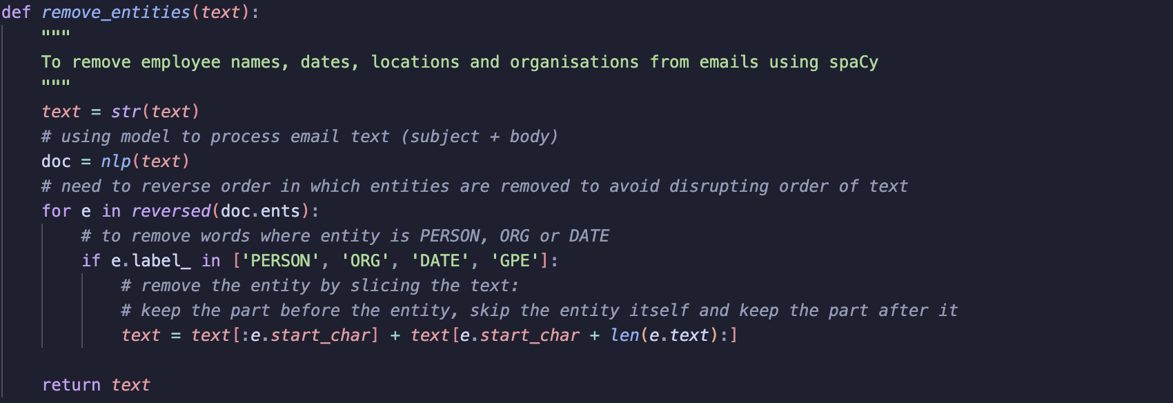
Step 2: Named Entity Recognition (NER)

Emails often contain employee names, organisations, locations and dates. For my project, this information is not relevant to my end goal and so thought it best to remove them to avoid unnecessary information. To do this, I used spaCy’s NER to find and remove words related to these entities PERSON, ORG, GPE and DATE before passing data to the TF-IDF vectoriser.

NER works based on positions of tokens within a document. SpaCy automatically tokenises the text into tokens. Each token is assigned a start and end character, essentially marking their position in the document.

For example, lets say we have the email:

John from Enron is meeting with Jane Doe on January 22nd

If you process the email using nlp(email) via spaCy, it detects the entities like this:

Token	Entity Label	Starting Character	Ending Character
John	PERSON	0	3
Enron	ORG	10	14
Jane Doe	PERSON	28	36
January 22nd	DATE	41	52

Since NER works by identifying entities at certain positions, we need to be careful about removing them as removing a single entity shifts the position of other tokens which could cause spaCy to misidentify other entities.

For instance, if we first remove John the remaining text looks like this:

from ENRON is meeting with Jane Doe on January 22nd

Now, the remaining token positions no longer match the original start and end characters, which could result in NER missing the other entities.

To solve this, I reversed the order in which entities are removed, starting with the last entity found in a document and then working backwards.

Step 3: Preparing a Tokeniser

Next, I prepared a custom tokeniser to pass to the TF-IDF vectoriser. A tokeniser is a function that tells the vectoriser how to process given text and split it into tokens. It can also include some cleaning of text before it is passed to the vectoriser.

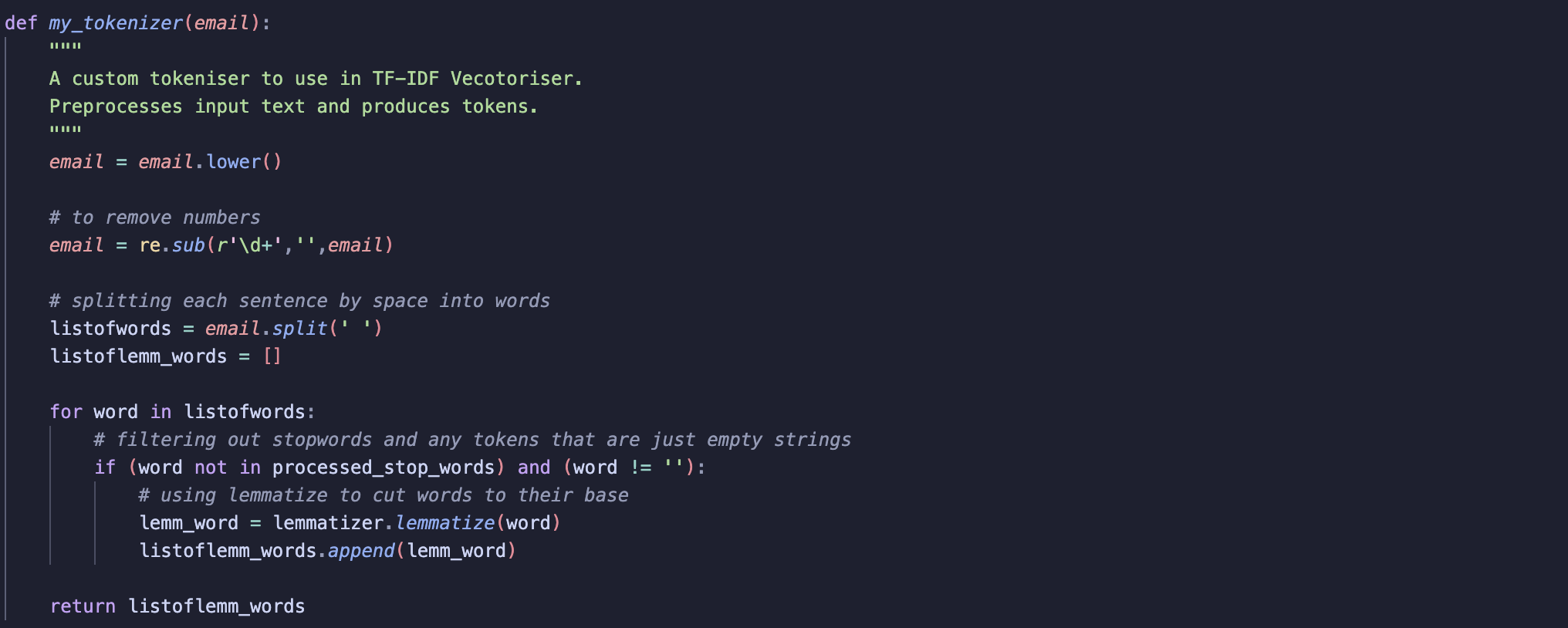
In my case, my tokeniser:

Converts all text to lowercase: Without this words that are capitalised and those that are in lowercase would be treated as different tokens. By converting all text to lowercase, we ensure a word is treated the same regardless of the casing. For example, “Email” and “email” would now be treated as the same token.
Removing numbers: Removes any remaining digits in an email.
Splits an email into tokens.
Removes stop words and empty strings.
Lemamtizes words: Lemmatization is basically where words are cut to their root. For example, “emailing” and “emails” becomes “email”. This helps to standardise the data and can reduce the feature space by grouping different variations of words to one. The screenshot below shows how to instantiate the wordnet lemmatizer.

The TF-IDF vectoriser will then use these tokens and represent them in a numerical format ready for further processing.

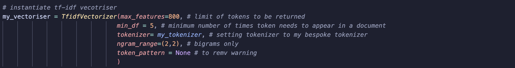
Step 4: using TF-IDF

The next step is to instantiate the TF-IDF Vectoriser, when doing this you can set some parameters to refine the output.

Parameters explained:

max_features: Limits the number of tokens to be returned. This is handy when it comes to reducing the feature space and focusing on the most relevant words.
min_df: Sets a minimum number of times a token needs to appear in a document to be considered. I set this to 5 meaning a token must appear in 5 documents before it becomes part of the feature space.
tokenizer: By default, TF-IDF uses its own tokeniser. Since I built a custom one, I pass the name of my tokeniser.
ngram_range: controls the size of tokens. I thought it best to return bigrams as features as pairs of words will help to give greater context to the tokens.

After this, we can then fit the vectoriser to the data and transform it.

Once the vectoriser is fitted and the transformation is complete, we get the following outputs:

get_feature_names_out(): This returns a list of all the tokens that the vectoriser has found.
text_transform.toarray(): Since the TF-IDF vectoriser returns a sparse matrix, we use toarray()to convert the sparse matrix into an array.

To display the results clearly, we can create a dataframe where the columns are tokens, rows represents single emails and values are the TF-IDF scores.

Results

To start, I wanted to see the most frequent tokens in the dataset to understand what appears most often in the emails and to see if there any themes emerging in the data.

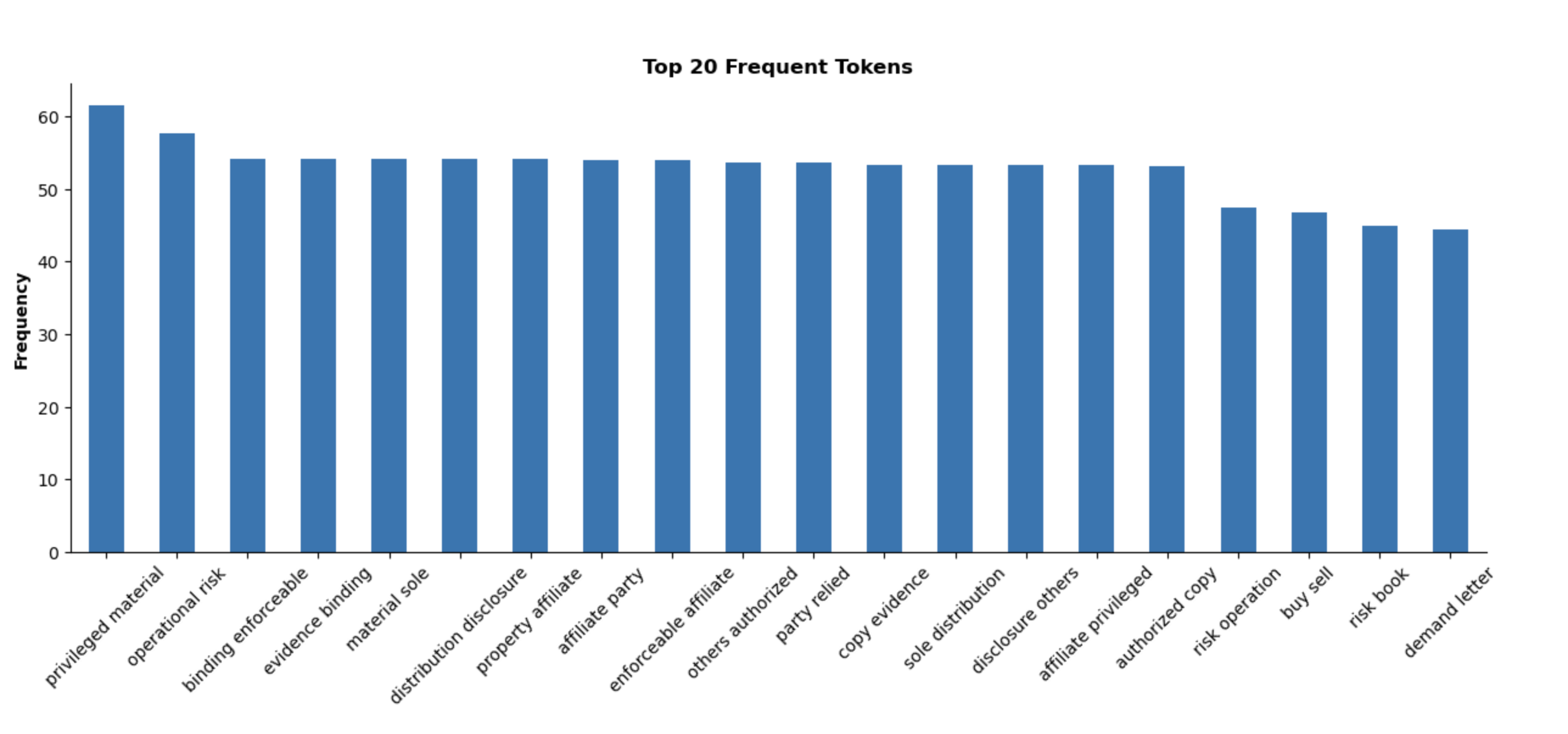
Already we can see some themes in the terms:

Legal Terms

Terms such as “privileged material”, “binding enforceable”, “distribution disclosure”, “evidence binding”, “affiliate privileged”.
Suggests many emails seem to focus on confidentiality and legal compliance/agreements.

Risk and Financial Terms

Terms like “operational risk”, “risk operation”, “risk book”, “buy sell”.
Suggests many emails discuss risk management and financial transactions.

After reading about Enron, these findings seem to align. The company faced issues in risky trading, compliance issues and even dodgy affiliations to hide losses. High scoring terms in the dataset seems to revolve around these issues and so I moved to topic modelling for further insights.

Topic modelling using LDA

Topic modelling is a method used to find topics in a collection of documents. Topic modelling is unsupervised, meaning the model automatically groups words into topics based on the data.

For this project, I use Latent Dirilech Allocation (LDA).

LDA follows a probabilistic approach to grouping documents. Initially each token in a document is classed as a random topic. The model then reassigns tokens to topics based on the probability that the token belongs to a certain topic. Like with other machine learning models, this process is repeated until the model converges.

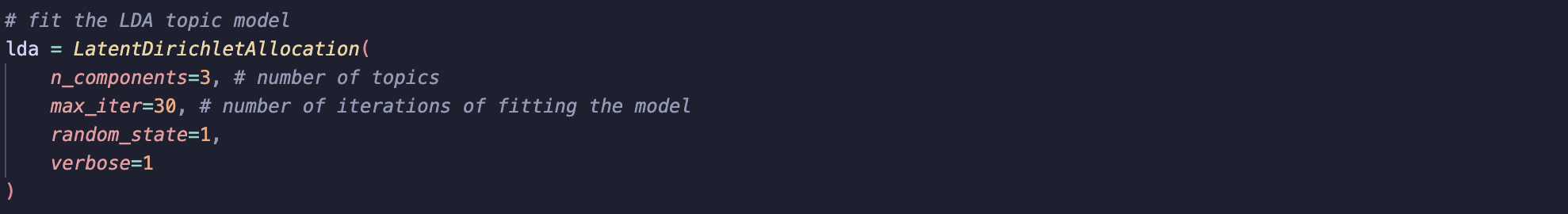
First, we have to instantiate LDA:

Then fit it to the transformed text:

So far, we have seen the most common words in the dataset and assumed some possible themes based on the most frequent tokens. Let’s take a look at the results:

Topic #1: Finance

Terms: risk book demand letter global market cash flow associate analyst west desk read directory real estate super bowl natural analysis.

This topic revolves around finance and trading, with key terms like risk, book, and cash flow. We also see terms like real estate and analysis appear for the first topic, perhaps this could be some sort of investments. Term super bowl is interesting, this could be some noise or indicate some sort of affiliation with a financial impact perhaps some advertising or a partnership.

Topic #2: Operations

Terms: operational risk risk operation mark calendar greatly appreciated yahoo yahoo shipping handling short notice security approver advise interest listed security

The second topic seems to focus on operations, terms like “shipping”, “handling”, and “short notice” suggest supply chain problems. The frequent occurrence of “risk” suggests potential issues in regard to operations or security.

Topic #3: Legal

Terms: privileged material property affiliate evidence binding binding enforceable material sole distribution disclosure affiliate party enforceable affiliate others authorised party relied

The third topic points to legal and compliance concerns, with terms like “binding” and “affiliate” suggest it involves contracts. “Disclosure” suggests confidentiality, possibly related to compliance.

Summary

In this post, I introduced the process of vectorising data with TF-IDF, including code snippets and a some preliminary insights into the ENRON dataset. Due to the promising results of TF-IDF, the next step will be to explore word embeddings to see if we can achieve even better results.

While the original plan for this project was to identify groupings in corporate emails, the results from TF-IDF and topic modelling suggest that we could also gain valuable insights into Enron’s downfall using NLP. I am excited to see what sort of insights word embeddings will uncover!