Email Genie: BERT 🤖

In the previous post, I explored using Word2Vec’s Skip-Gram to generate embeddings for emails in the Enron dataset. While Word2Vec was able to capture some semantic relationships, such as grouping financial, operational and legal terms together, it struggled with understanding context of words with multiple meanings, like “risk” or “market”.
In this blog post, I will try a different approach by using a transformer model (BERT) to create the embeddings. Transformers are better at capturing the relationships between words and have a deeper network that can pick up more nuanced relationships, especially for words with multiple meanings.
Transformers
Transformers are the next step up from Word2Vec. While Word2Vec can generate word embeddings that capture some semantic relationships, it’s limited by a fixed context window. This means it only considers a few words before and after the target word, which can lead to rigid embeddings that don’t adapt well to different meanings in different sentences.
Transformers are different as they crate context-aware embeddings, let’s revisit the same example:
-
Document A: “Today, I went to the bank to deposit some money”
-
Document B: “Today, I sat by the bank of a river and had lunch”
Word2Vec generates only a single embedding for “bank”. As a result, its vector would likely be positioned somewhere between the finance and nature clusters in the vector space. On the other hand, transformers generate different embeddings for each instance of “bank” as seen in the graph in the previous post. Using transformers to create the embeddings for this project can help to better understand the nuances in the emails which Word2Vec missed.
Encoders VS Decoders
There are two important parts to transformers: encoders and decoders. When transformers first came out, most thought both were necessary to perform tasks. After some time, it became clear that transformers could be made up of both encoders and decoders but also work with just an encoder or decoder.
What are Encoders?
Encoders are designed to read and understand text by generating context-based embeddings. Encoder based transformers include models like BERT, where the main purpose is to understand the semantics of given text.
What are Decoders?
Decoders are designed to generate text by predicting the next word in a sentence based on the context of previously generated words. Models like ChatGPT are a decoder-based transformer and these types of models are better suited to more creative tasks like completing sentences or rewording paragraphs.
Since my project is based on understanding the semantics of the emails and generate embeddings that capture the most context, I focused on encoder-only transformers.
BERT
The purpose of BERT is to create context-based embeddings, where similar words used in similar contexts have similar vectors. Unlike Word2Vec that generates static word embeddings, BERT understands the meaning of words and so is great for tasks requiring semantic similarity or classification.
How does BERT work?
BERT is a pre-trained model, trained on millions of documents to understand the context of words by considering not just their position but also their meaning within the sentence.
Below, I have drafted out a diagram to help understand how BERT works.
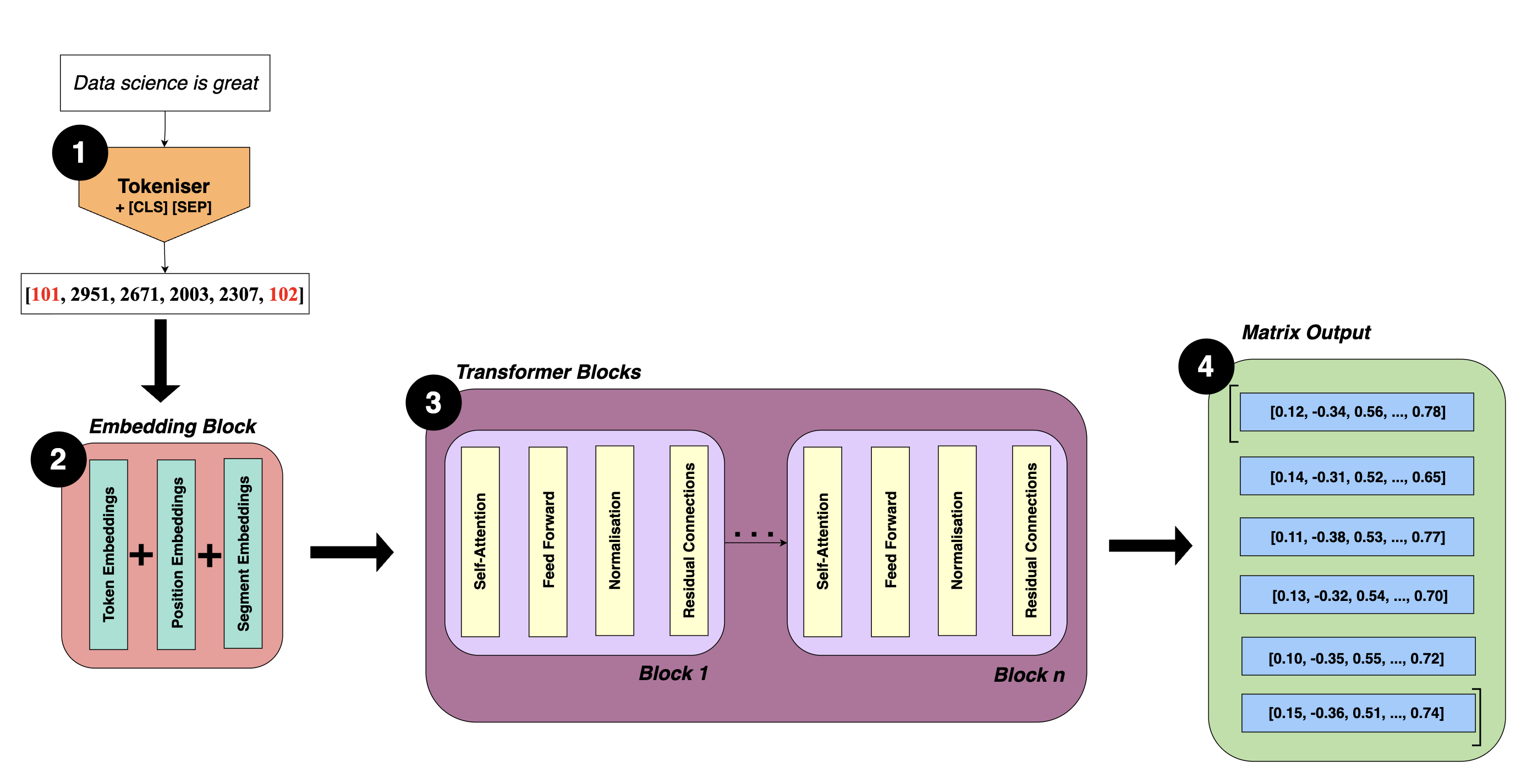
Step 1: Tokenising Input Data
Before BERT can process text, the input must be tokenised. Tokenisation is the process of breaking down the input into smaller parts, either individual words or groups of words. Each part is then converted into a token ID, so the input text is now represented as a vector.
Each token ID corresponds to a token in BERT’s existing vocabulary, since BERT is a pre-trained model. BERT uses its own tokeniser from the transformers library, I touch on this later in the post.
Tokenisation also introduces some special tokens to help the model better understand structure of given text:
-
[CLS]: Marks the beginning of input -
[SEP]: Acts as a separator to differentiate different parts of the input, for example separating out questions from contexts.
For the input sentence: “Data science is great”
Tokens: [[CLS], “data”, “science”, “is”, “great”, [SEP]]
Token IDs: [101, 2951, 2671, 2003, 2307, 102]
Step 2: Embedding Block
After tokenisation, the list of token IDs are passed to the embedding block where the token IDs are transformed into embeddings. It is called an embedding block because it combines three types of embeddings to produce context-based embeddings:
1. Token Embeddings
Each token ID is mapped using a lookup table to a learned vector. These vectors capture the meaning of each token.
| Token | Embedding |
|---|---|
| [CLS] | [0.2, 0.3, 0.4] |
| data | [0.1, 0.2, 0.7] |
| science | [0.5, 0.6, 0.9] |
| is | [0.8, 0.2, 0.1] |
| great | [0.3, 0.6, 0.7] |
| [SEP] | [0.0, 0.9, 0.1] |
2. Position Embeddings
Positioning of tokens in a document is important as meaning can change depending on order. For example:
-
“Data science is great”
-
“Data science is not so great”
Token embeddings alone only tell the model what words are present in the corpus: [“data”, “science”, “is”, “great”, “not”, “so”]
Position embeddings tell BERT where each appears in the sequence of tokens and so allows the model to understand that not becomes before great changing the sentiment. In BERT, each position has its own learned position embedding vector, these position embeddings are added to the token embeddings so now embeddings capture what each token is and where each token is.
So now the embeddings look like:
| Token | Token Embedding | Position Embedding | Final Embedding |
|---|---|---|---|
| [CLS] | [0.1, 0.2, 0.3] | [0.0, 0.0, 0.0] | [0.1, 0.2, 0.3] |
| data | [0.4, 0.5, 0.6] | [0.1, 0.1, 0.1] | [0.5, 0.6, 0.7] |
| science | [0.7, 0.8, 0.9] | [0.2, 0.2, 0.2] | [0.9, 1.0, 1.1] |
| is | [0.3, 0.3, 0.4] | [0.3, 0.3, 0.3] | [0.6, 0.6, 0.7] |
| great | [0.5, 0.6, 0.7] | [0.4, 0.4, 0.4] | [0.9, 1.0, 1.1] |
| [SEP] | [0.0, 0.1, 0.2] | [0.5, 0.5, 0.5] | [0.5, 0.6, 0.7] |
3. Segment Embeddings
BERT also uses segment embeddings. These embeddings are only relevant for inputs where there are pairs of sentences like question and answer pairs. Segment embeddings help BERT understand which part of the input belongs to which sentence.
For example, input could be:
Sentence A: “What do you think of data science?”
Sentence B: “Data science is great”
In this case:
-
The tokens from sentence A will have a segment embedding of 0.
-
The tokens from sentence B will have a segment embedding of 1.
If the input is a single segment (like the one in our diagram), the segment embedding is 0 for all tokens.
Step 3: Transformer Blocks
Once the embeddings are ready, they passed to a number of transformer encoder blocks, typically BERT has 12. Each transformer block is made up of:
Self-Attention
Self-Attention allows BERT to understand how each word in a sentence relates to every other word, regardless of distance.
The model calculates attention scores between each pair of tokens. These scores help determine how much attention the model should give to other tokens when encoding. I like to think of attention scores like a multiplier telling the model how important a certain word is to each other word.
For example:
“The bird didn’t catch the worm because it was too tired”
Here, “it” could refer to “bird” or “worm”, if “bird” has a higher attention score than “worm” and so learns “it” is most likely referring to “bird”.
Feed Forward
After self-attention, each token is then passed through a small fully connected neural network. This network helps the model learn more complex features such as:
-
Whether a token is a subject, object or verb?
-
If the token is a named entity like an organisation or person?
-
If the token carries any sentiment?
Note: It’s called Feed Forward since the model is using what it has learnt during training to enhance it’s understanding.
Normalisation
Layer normalisation is used to stabilise and increase training speed. It works by scaling inputs to each layer in the block like self-attention and feed forward networks so that the mean is 0 and variance is 1 for each token’s embedding vector.
The purpose of this is to prevent exploding or vanishing gradients which is a risk to deep models like BERT where there are a lot of layers. Normalising the output of each sublayer ensures gradients are more stable, making it more likely for the model to reach convergence.
Residual Connections
Vanishing gradients are a common issue in deep networks like BERT as the gradients can shrink a lot as they pass through all layers. When this happens, weight updates are tiny and learning is slow.
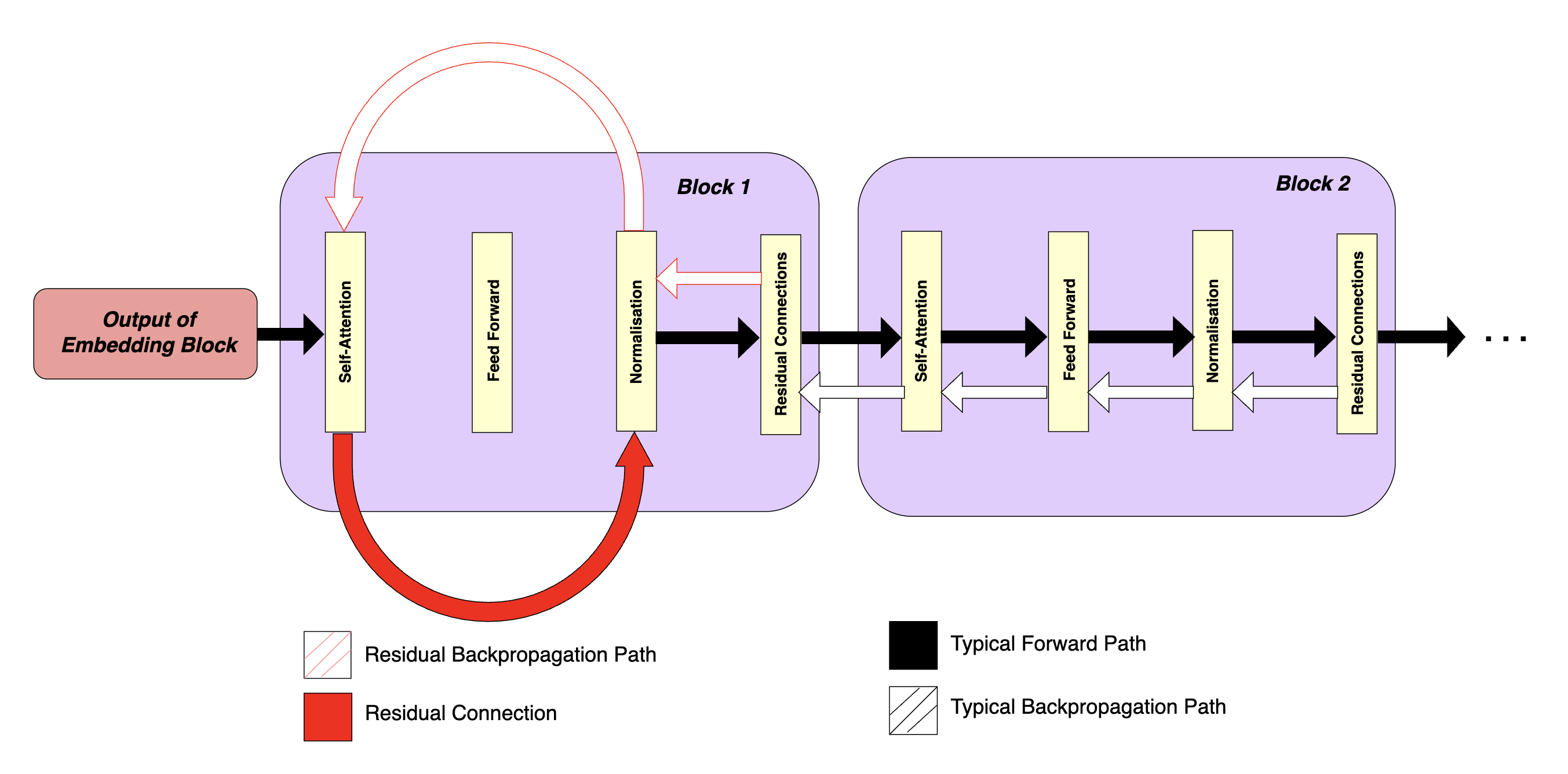
Residual connections (shown red in block 1) address this issue by adding shortcuts around sublayers in a block. These shortcuts create another path for the gradient to flow back through and allows it to bypass some of the transformations which could cause it the vanish. As a result, the gradient doesn’t have to pass through as many layers and so retains its size.
In block 2, the normal feedforward flow passes through each sublayer one by one. During backpropagation, the gradient flows backward through the same sublayers to update weights. Without residual connections, the gradient must pass through all these layers, which increases the chance it will shrink and slow learning.
Step 4: Matrix Output
Once the data has passed through all transformer blocks, the final output is a matrix of embeddings.
Each row of the matrix is a high-dimensional vector representing a single token.
So for: “Data science is great.”
The output will be something like:
[CLS] → [0.12, -0.34, 0.56, ..., 0.78]
data → [0.14, -0.31, 0.52, ..., 0.65]
science → [0.11, -0.38, 0.53, ..., 0.77]
is → [0.13, -0.32, 0.54, ..., 0.70]
great → [0.10, -0.35, 0.55, ..., 0.72]
[SEP] → [0.15, -0.36, 0.51, ..., 0.74]
To get a single embedding for a given sentence, you need to pool these embeddings. Pooling is the process of combining all token embeddings into a single vector.
There are different pooling methods each combine the embeddings in different ways. For my project, I used mean pooling which I talk about in the next section!
Implementing BERT
Since I am running this project on my computer and working with a small dataset, I chose to use DistilBERT instead of BERT. DistilBERT is basically a lighter and faster version of BERT.
Step 1: Preparing Text
Like the other methods, the first step is to combine the subject and body of each email and to use NER to remove any mentions of employee names, organisations and dates to reduce noise.
Step 2: Tokenising Text
Before passing the emails into the model, the text must be tokenised. For this, I use the DistilBERT tokeniser from the Hugging Face transformers library.

One important note is that the tokeniser has a maximum output limit of 512 tokens. Some emails in the dataset are longer than this and so I chunked the emails into smaller parts to handle this. Chunking basically means splitting a long email into smaller chunks so that each chunk fits within the model’s token limit.
Let’s walk through my function step by step:
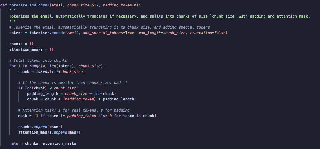
For a given email I first tokenise the email using encode which returns a list of token IDs. I set add_special_tokens=True so that special tokens like [CLS] and [SEP] are added automatically. These special tokens help the model understand where the email starts and ends. I also set truncation = False as I will be chunking the emails not truncating them to fit the token limit.
Note: A single token does not always correspond to a single word. Sometimes multiple words can be combined into one token, and sometimes a single word can be split into multiple tokens
The next step is to chunk the tokenised email.
To do this, I iterate through the list of token IDs with an increment of chunk_size. I create a chunk by slicing the token list from i to i + chunk_size, making sure each chunk contains up to chunk_size tokens.
Once a chunk is created, if it is smaller than the chunk_size, I pad it with the padding token to ensure all chunks are of size 512.
I then create an attention mask for each chunk. The attention mask is a list that tells the model which tokens are real (1), and which are padding (0). This helps the model to focus on the meaningful parts.
Step 3: Create tensor objects
The DistilBERT transformer requires inputs to be in the form of tensor objects.
To do this, I use PyTorch (torch) to convert both the tokenised emails and attention masks into tensors.

After that, I create a TensorDataset to help organise the data, speed up training and avoid errors related to object types.

Step 4: Creating the embeddings
For generating the embeddings, I’m using the pre-trained weights of DistilBERT. This means I’m just passing each email through the DistilBERT model and extracting the embeddings.
I load the DistilBERT model and set it to model.eval(), this lets the model know that it is in evaluation mode and so no updates will be made to the weights and to not do dropout.

Since I don’t have access to a GPU, I batch the data using DataLoader from PyTorch.

Next, I iterate through each batch. I use torch.no_grad() to ensure no gradients are calculated since we are not updating any weights.
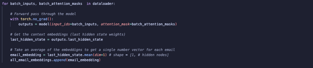
I pass the tensor inputs through the model and access the output from the last hidden layer, which contains the embeddings. As mentioned earlier, DistilBERT generates a separate embedding for each token in the email, and since the embeddings have over 700 dimensions, this can result in a large number of embeddings. To reduce this to a fixed-size vector per email, I used mean pooling. Mean pooling takes the average of all token embeddings so now I have a single embedding per email.
Note: After evaluating the embeddings, I realised that mean pooling may not be the best method to use. This is because mean pooling treats every token the same meaning padding tokens contribute just as much as meaningful tokens. This could affect the quality of the embeddings, especially when using them to assess semantic similarity. Ideally, I would have experimented with different pooling methods such as weighted pooling, but each time I tried, my kernel crashed.
Step 5: Unbatch and save the embeddings
Before saving the embeddings, I needed to unbatch them back into individual email embeddings:

After this I then saved the embeddings:

Results and Evaluation
UMAP
UMAP is a dimensionality reduction technique, similar to t-SNE. I thought it best to visualise the embeddings by applying UMAP to see whether any clustering exists within the dataset.
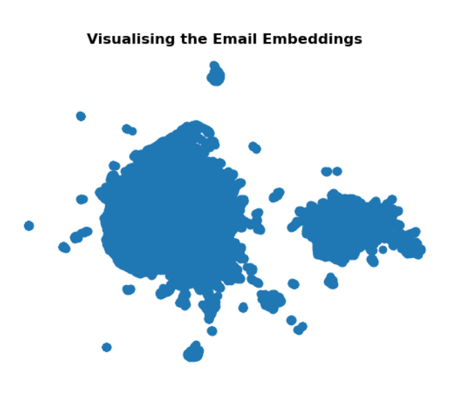
From the UMAP plot, there are two main clusters. One was significantly larger, almost double the size of the other. Although these clusters seem somewhat well separated, there is noticeable noise around each cluster.
To try improve results, I played around with some of the UMAP parameters:
-
n_neighbors=15: This controls how many neighbouring points the model considers. The higher this value is the more broad the insights are. -
min_dist=0.5: Determines how close points are together, a lower value results in tighter clusters; a higher value spreads them out more. -
metric='cosine': Metric to measure similarity between embeddings -
n_components=2: This sets the output dimensionality. Since I’m working with Matplotlib, I reduced it to 2D for plotting.
Despite tuning these parameters, the structure of the clusters didn’t improve significantly. As a result, I thought it best to see how well the embeddings group similar emails together.
Assessing Embedding Similarity
To evaluate the quality of the BERT embeddings, I calculated a similarity matrix using cosine similarity. Given the large number of emails, I randomly sampled batches of 10 emails at a time and assessed the results. For each sampled email, I returned the top 2 most similar emails and the most dissimilar ones.
Considering the noisiness of the Enron email dataset, out-of-the-box BERT doesn’t seem to perform too poorly on real-world emails. The model does show some meaningful grouping based on topic and tone — for example, legal and finance-related emails often appear together, and casual or personal messages (e.g., birthday wishes) also tend to cluster.
To see the results in more detail, please refer to the notebook here (to be made public when project is complete).
This suggested that pretrained BERT alone may not be ideal for capturing the nuances of in the ENRON dataset. Perhaps it would be better to move to Sentence Transformers, which are more effective at capturing semantics at the sentence level rather than just at the token level.
Clustering
Despite the not so promising results for my embeddings, I still was curious to see how well they will do in clustering. Using the UMAP plot as a visual reference, I applied both K-Means and DBSCAN to the reduced embeddings.
K-means
After experimenting with different values for k, I found that k = 3 produced the best results in my opinion.
Inertia: 167,169
Inertia measures how tightly the samples are clustered around their centroids — lower values indicate more compact clusters.
A score of 167000 is relatively high, suggesting that the clusters aren’t tight. However, given that the embeddings come from an out-of-the-box BERT model and the data is quite noisy (even after preprocessing), this isn’t a surprise.
Silhouette Score: 0.12
The silhouette score reflects how similar a point is to its own cluster compared to others. A score of 0.12 is on the lower side, again highlighting that the clusters are not well-separated. But since I didn’t fine-tune BERT to the data, a low score makes sense.
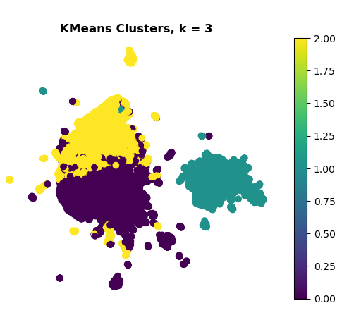
-
One cluster, positioned clearly on the right stands out as well-separated.
-
The other two clusters on the left, show significant overlap, this suggests the model struggles to distinguish between these groups.
DBSCAN
DBSCAN is a clustering algorithm that identifies groups based on density rather than distance, unlike K-Means. I decided to try DBSCAN because it can be more effective in handling noise, which we saw in K-Means and UMAP plots
To evaluate results of DBSCAN, I counted the number data points in each cluster found rather than using traditional clustering metrics. This was because the 2D plot of the DBSCAN results did not show strong groupings (see below).
Cluster Label -1: 6,518 points
- These are points that DBSCAN labelled as noise. This means they didn’t meet the density requirements to be assigned to any cluster, based on parameters I set (after hyper-tuning as much as possible).
Cluster Label 0: 29,127 points
- Majority of the datapoints belong to Cluster 0. This suggests that no strong or distinct groupings were found and that the differences between points are likely subtle.
Cluster Label 1: 9 points
- Only 9 points were dense enough to be grouped together and separate from the main cluster. Since there is such a small number of data points in this cluster, I doubt it has much semantic meaning.
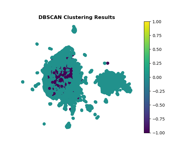
DBSCAN did not help much in making meaningful clusters, the dominance of a single clusters and high number of points categorised as noise makes me think the quality of the embeddings needs to be much better. So, I decided not to go ahead with exploring other clustering methods as I think I need to first improve the quality of the embeddings.
Summary
In this post, I introduced transformers and explained how BERT generates context-based embeddings, demonstrating how to use it with HuggingFace’s library on the Enron dataset. Pretrained BERT struggled to separate emails, as shown by weak clustering results. I think it may be best to explore Sentence Transformers to create the embeddings, they are more lightweight than BERT meaning I don’t have to worry about kernel crashing and they’re made to capture semantic meaning more effectively.