Email Genie: Vector Databases 🗄️

In my last post, I explored different modelling techniques in an attempt to build a classifier for emails. Despite trying a range of traditional methods and even fine-tuning a DistilBERT model, the results weren’t great… all models struggled and performance was less than 70%. I think the main reason for this was either: lack of data in the labelled dataset for the model to learn well or lack of separation in vector space between the embeddings.

So, I decided to change the scope of my project to vector databases and similarity search! Vector databases have been on my list of things to try for a while and instead of forcing emails into predefined labels, I thought what if we could explore the dataset more naturally?

The Enron email dataset is messy, but offers lots of insights. It includes everything from business and trading activity to casual office chat. With a vector database, we can search by meaning rather than exact keywords, so we can search for themes like:

Corporate culture: bonuses, employee performance
Energy trading: market risk, pricing
Crisis times: bankruptcies, resignations, investigations
Day-to-day operations: weekend updates, office parties, drinks

Let’s first recap what vector embeddings are and get a better understanding of what vector databases are and how they work!

Vector Databases

Before diving into Vector Databases, I thought it a good idea to give a bit of a recap to vector embeddings and what they represent using a simple example:

Sentence	Embedding
Today was a rainy day	[0.88, -0.45, 0.61, 0.33, -0.27]
It was a rainy afternoon	[0.92, -0.47, 0.07, 0.31, 0.25]
I like to play tennis in the park	[0.05, 0.90, 0.85, 0.36, 0.42]

Embeddings are a way to represent unstructured data like text and even images by an array of numbers. In the example above, we’ve created embeddings for three sentences. There are many different embedding models we could use for this, to learn more about the different types, you can revisit some of the previous posts in the Email Genie series.

Sentences with similar meanings have similar embeddings. In our example, sentences 1 and 2 are both about rain, notice how their first numbers (0.88 and 0.92) are close to each other. Sentence 3, however, doesn’t mention the rain at all, and its first number is much lower (0.05), showing it’s less related in meaning to the first two.

Each number in the array represents a certain feature, its value signals how strongly the data relates to that feature. Values closer to 1 indicate a stronger relationship and values closer to 0 indicate a weak relationship. Knowing this, we can say that vector embeddings which are grouped closely together have similar meanings. This idea is at the core of how vector databases work, they store these embeddings and when given an input, find and return the items most like it.

Now that we understand embeddings, let’s see how vector databases use them to do semantic search!

What are Vector Databases?

Databases are used to store and query data. The most common type many have come across is the relational database, where data is organised into tables with rows and columns. Each row has a unique primary key and we can query the data using SQL.

For example, to return all rows where the colour is pink:

SELECT * FROM MY_TABLE WHERE LOWER(COLOUR)= 'pink';

This works perfectly for structured data (data that can be defined by columns like dates, amounts, short strings).

However, unstructured data like free text, images or audio is a bit trickier. If we want to search through sentences (like those in the earlier example) to find ones with a similar meaning, SQL queries won’t work. SQL can only match like to like, it has no understanding of the meaning behind the data.

This is where vector databases come in. Instead of storing text in its raw form, they store vector embeddings. As we discussed earlier, embeddings represent data in vector space where similar items are close together.

Because of this, vector databases can perform semantic search, returning results ranked by meaning, not just exact matches. They can answer queries like “show me emails about bankruptcies” even if the word “bankruptcies” never appears in the text, something a traditional relational database can’t do.

How Is Data Stored?

When you store data in a vector database, you can’t just write to the database and dump the data there, you need to:

1. Convert the data into embeddings

As discussed, all data must be represented as a vector. To do this we use an embedding model to create the embeddings.

2. Metadata

Usually store some metadata alongside the embeddings, includes things like a timestamp or date, email id and sender id (in this case), and any other information which could be important to the project.

3. Vector Indexing

Just like other databases use primary keys to speed up searches. Vector databases also use indexes but not the traditional kind since they are not matching exact values.

A vector index organises vectors so that the database can find vectors that are most similar to a given input. Instead of scanning the entire dataset, the vector index narrows the search to the most relevant areas of the vector space. This is what makes retrieval so quick!

To do this, we use an approach called Approximate Nearest Neighbour (ANN) search. ANN methods organise the vector data so similar vectors are grouped together. There are different ANN techniques to choose from:

a). Flat Index

A brute-force approach for vector search. For a query vector, it calculates the similarity metric with every vector in the dataset and returns the top n closest vectors. It is simple and precise but not efficient for large datasets since each vector is compared to the query vector.

b). HNSW (Hierarchical Navigable Small World graphs)

HNSW essentially uses multiple layers of maps to search the vector space. Understanding how exactly HNSW works took me a while to get my head around… For me, it helped to start with the concept of skip lists.

Suppose we have a sequence: 1, 2, 3, …, 9, and we are querying for the number 8.

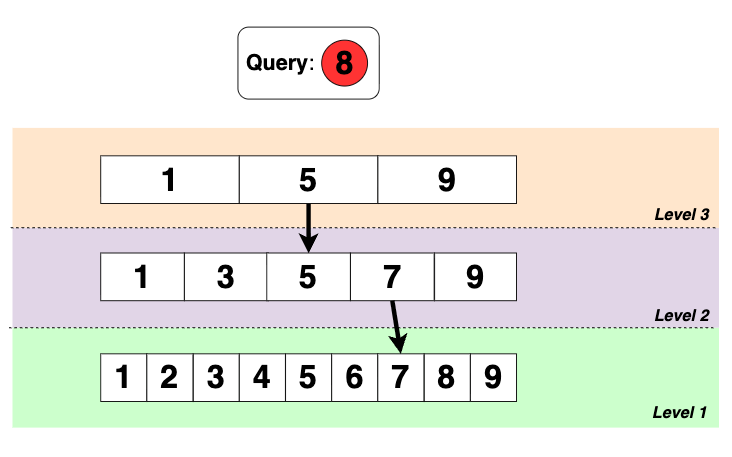
The brute force approach is to iterate over each number until reaching 8, this isn’t efficient especially with large datasets. Skipped linked lists speeds things up by using multiple layers.

Search process

Start at the top level (Level 3). Move forward until the next number is larger than the query.
Drop down to the next level at the last node where query is greater than.
Repeat until the query number is reached.

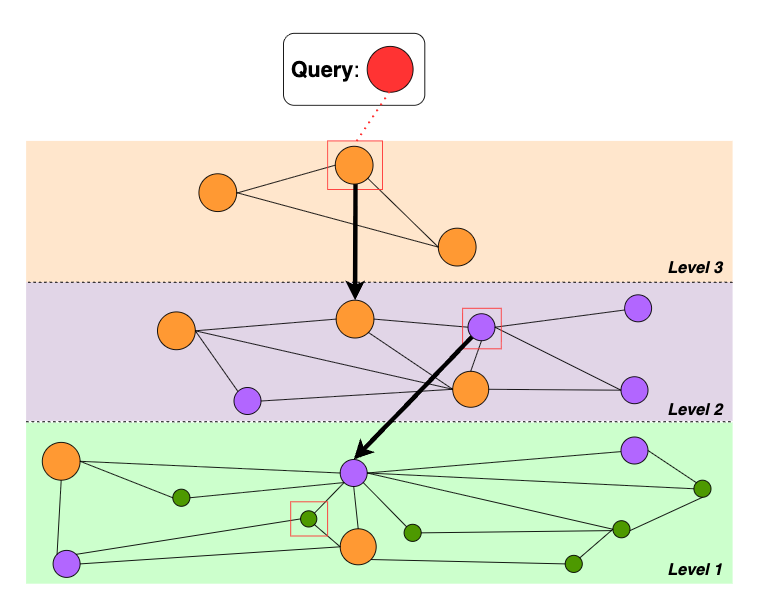
For HNSW, the concept is the same:

Level 3 (highest layer)
- A zoomed-out map
- Each point is connected to a few other points
- Start at a random node and use a similarity metric to find the region closest to the query and drop to the next layer
Level 2 (middle layer)
- A more detailed map showing more nodes and connections
- Repeat similarity calculates to find nodes closest to the query
- Drop down again
Level 0 (bottom layer)
- The most detailed map, showing all nodes and connections
- Here, we can find the exact nearest neighbours of the query

c). IVF (Inverted File)

IVF first groups vectors into k clusters (called buckets) using a clustering algorithm like k-means. For a given query vector, it calculates which bucket is closest using a similarity metric like cosine similarity. Only vectors in those clusters are searched reducing the total search space.

Similarity Search

Now that our vectors are grouped by similarity, we can now use similarity search to return vectors most like the input. Here is how it works:

1. Convert your search query into a vector

Just like with the data in the vector database, the search input is passed through the same embedding mode turning the input query into a vector.

2. Search the vector index for nearest neighbours

The vector databases don’t do a one-by-one comparison of every vector to the search vector. Instead, it uses vector indexes to quickly find vectors that are close in semantic meaning.

3. Calculate similarity scores

For all candidate vectors found by the index, the database calculates a similarity score. There are lots of different ways to do this, there are the most common:

Cosine similarity: compares the angle between vectors.
Dot product: measures how much the vectors point in the same direction.
Euclidean distance: measures straight-line distance in vector space.

Vectors with higher similarity scores are more related in meaning.

4. Return top results with metadata

The database returns the top n most similar vectors along with their metadata, ready for evaluation. In cases where you have a labelled dataset, you could use majority voting on the labels of the returned vectors to determine the label of the input query. This was an option I considered for my project but ultimately decided to limit my project to semantic search. I did this as I had concerns over the quality of my embeddings. Further down in the post I explain why this is.

Implementation

Note: My implementation wasn’t as smooth as the steps below, I did iterate over the process quite a few times in an attempt to get results as strong as possible!

Step 1: Choosing a Vector Database

I considered two popular options: FAISS and Pinecone. I chose FAISS because it’s fast, easy to set up, and low maintenance. Ideal for quick development and integration into a web app. Plus, it’s open-source, lightweight, and gives me full control for experimenting with different index types!

Step 2: Load Dataset

After installing FAISS on my conda environment, I loaded in my dataset and prepared it data for the next step.

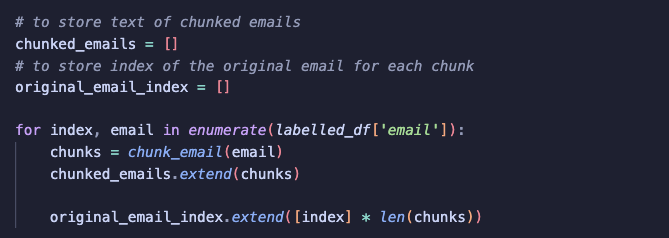
Step 3: Chunk Emails

Previously, when I used Sentence Transformers, I didn’t chunk my embeddings. However, since my project focuses on similarity search, I thought chunking emails was important.

From my research so far and the nature of emails in general, its common for emails to fall into multiple categories. Chunking helps handle situations where one part of an email is financial, but another part is legal for example.

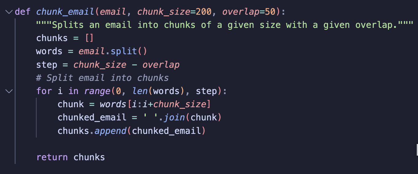
My chunking method is similar to how I chunked emails for BERT embeddings, with a few differences:

Include Overlap: I avoid strict boundaries between chunks so that context isn’t lost. Overlapping chunks can help preserve information that spans across multiple chunks.
No Masking/Tags/Padding: Sentence Transformers don’t need attention masks, special tokens like BERT’s [CLS], [SEP], or padding, as these are handled internally. So, I removed them.

I applied the chunking function to the lablled dataset:

Step 4: Create Embeddings

With the emails chunked, I then created embeddings using Sentence Transformers.

I chose a different, larger model than before because the smaller mini transformer was not returning good results. Since I’m only working with ~1,000 emails, I opted for a bigger model to generate higher-quality embeddings to improve the vector search.

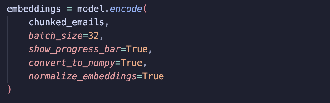
I also set the normalisation parameter when creating embeddings. Normalising embeddings helps improve similarity search by ensuring that comparisons like cosine similarity focus on the direction of the vectors rather than their magnitude. It also speeds up retrieval since cosine similarity becomes dot product when vectors are normalised.

Step 5: Build Index

Now it was time to move to the vector database!

In this project, I experimented with three common FAISS index types uisng their documentation as a guide:

Flat Index

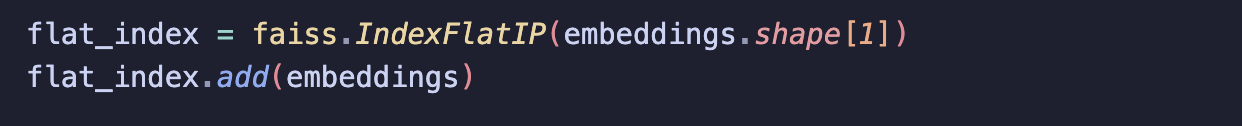
All index types need the dimension of the embeddings as input. After creating the index, I use add() to insert the embeddings. For the Flat index this just stores all vectors, ready for search.

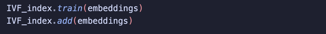
IVF Index

For IVF, I pass in the embedding dimension and set the similarity metric to cosine similarity. I also set the number of buckets to divide the embeddings into, for this project I chose 10.

Before adding embeddings to an IVF index, I needed to train the index so that it could calculate the cluster centres. Once trained, I added the embeddings to their clusters.

HNSW Graph Index

Like the other indexes, I pass the embedding dimension and set the similarity metric to cosine similarity. For HNSW, I also set the parameter M to 32, which controls the maximum number of connections per node. More connections per node increases accuracy but also requires more memory.

Here, add() inserts each embedding as a node in the graph and connects the nodes together to allow for search.

I used my labelled dataset to decide which index worked best for this project.

For the similarity metric, I chose cosine similarity instead of the default L2 (Euclidean) distance. Since embeddings have the same dimensions but can vary in magnitude, cosine similarity normalises the vectors and focuses solely on their direction, making semantic similarity more accurate.

Step 6: Evaluation

For evaluation, I decided to use the nearest neighbours approach.

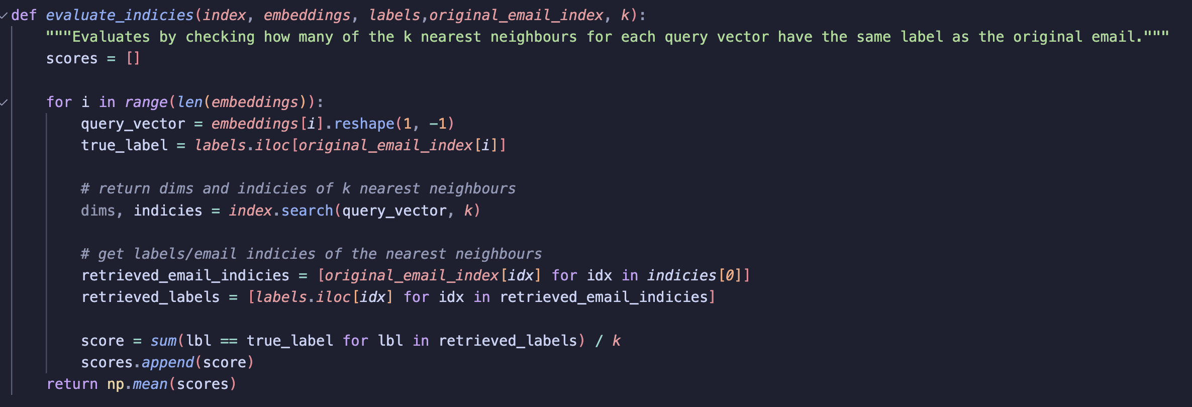
For each email, I retrieved the top 20 neighbours and stored the labels. I then compared how often these neighbours matched the label of the email being evaluated. This gave me a quantifiable measure of performance.

I chose k = 20 because evaluating a larger set of neighbours provides a more reliable picture of how well the embeddings cluster. By looking at multiple neighbours, I thought I would get a better gauge of the semantics within a given vector space.

Let’s take a look to see how the vector database performs.

Results

Overall, the results were not strong.

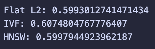
Even after all the tweaks I tried, performance still struggled to get pass 60%. Looking back, I think one of the main reasons is the choice I made to use out-of-the-box transformer models. Email data is messy and nuanced, and I probably needed something more tailored. Before I get into why, I also did a bit of qualitative testing:

I ran some semantic searches with a few keywords
I then manually checked the returned emails to see if they are actually relevant to the input
Since the main goal of this project was a web app where users could search across emails, this felt like a good real-world test

Unfortunately, the qualitative results were also weak. To understand why, I plotted the embeddings in 2D space. As I expected, there was a lot of overlap between different categories. The lack of distinct boundaries between the labels makes it harder to return semantically similar emails.

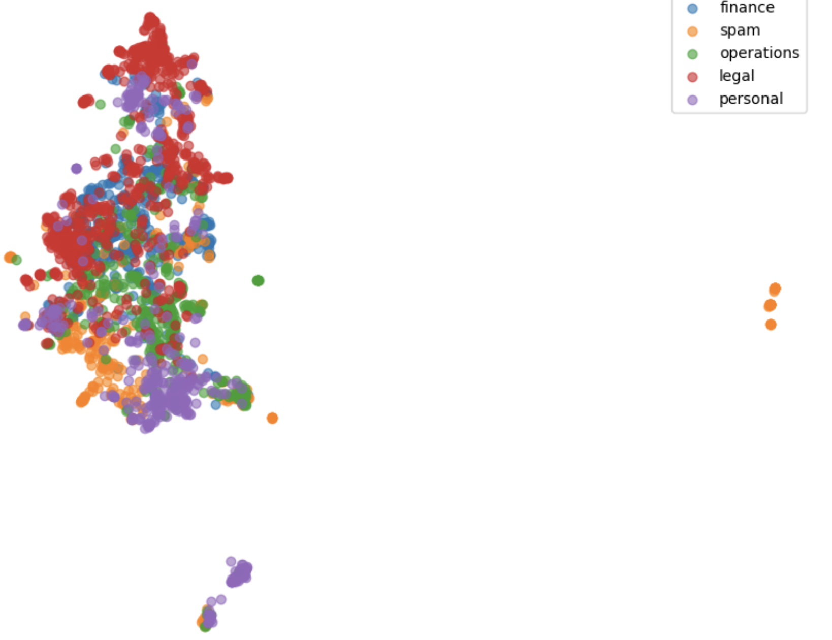
This kind of confirmed what’s been coming up again and again in this project, the embeddings just aren’t strong enough. The embeddings I’m using come from a pre-trained Sentence Transformer model, and I haven’t fine-tuned them at all. That means they’re pretty good at understanding general language, but struggle with the nuances of stuff like finance, legal or business/company jargon.

For this project this is an issue, since the end goal is for users to be able to search through the Enron emails to learn more about the company and its collapse. Without domain-specific fine-tuning, the model just isn’t picking up on the subtleties on what users would be searching.

Summary

After assessing the results, I was a bit defeated. I have spent a lot of time on this project and maybe was naïve to think that out-of-the-box embeddings would produce high-quality results for email text. I also overestimated what a vector database could do on its own.

Despite the temptation to stop here, I really want to see this project through. I’ve put a lot of effort into getting this far, and I feel there is a way to improve the results.

Over the next few weeks, my plan is to:

Limit the project to a smaller subset of emails (perhaps only the labelled ones)
Focus on improving the quality of embeddings so that the vector database can return meaningful results
If fine-tuning still proves to be an issue in terms of computing power, researching to see if there is a transformer trained on finance/corporate language exists. If so, perhaps investigate using this to improve my embeddings