Email Genie: Fine Tuning 📻

In my previous post, I wrote about vector databases. I explained how they work, shared implementation steps and my results. One recurring issue I noticed throughout the project was the quality of the embeddings. This was reflected in subpar results for both classification modelling and vector searches.

To address this, I fine-tuned a Sentence Transformer model on a subset of the Enron email dataset. The goal was to create embeddings that better understand the nuances of email text and corporate jargon, and in turn improve vector search.

In this post, I’ll walk you through the fine-tuning process and share what I learnt along the way! Let’s start with the process of fine-tuning embeddings and see what impact it had.

Fine-Tuning Embeddings

A few posts back, I explained how Sentence Transformers work. In this section, I’ll build on that. If you need a recap, refer to my earlier post: Sentence Transformers.

When fine-tuning Sentence Transformers, the main idea is to tell the model which emails are similar and which are not. This is done by creating sentence pairs:

Positive pairs: Two emails that are similar in meaning.
Negative pairs: Two emails that are not similar in meaning.

Positive pairs are given label 1 and negative pairs label 0. During training, these labels help update the model’s weights so that similar emails are pulled closer together in vector space, while unsimilar ones are pushed further apart.

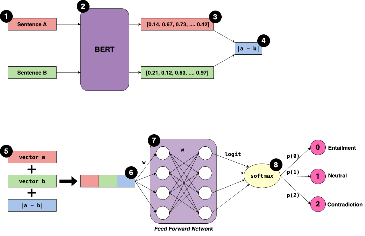
Looking at the diagram, the main trainable weights are in the transformer blocks of BERT. Since we are only using Sentence Transformer to create the embeddings we exit at step 3 (the output of the BERT model).

Fine-tuning “unfreezes” these weights and updates them using a loss function, allowing the model to adapt to input text. Out-of-the-box Sentence Transformers keep these weights fixed and so generate general purpose embeddings trained on massive datasets.

Implementation Steps for Fine-Tuning

For the full notebook, please refer to the GitHub repo (to be made public on completing the project). I also used Google Colab to complete fine-tuning for my embeddings as I needed access to a GPU.

Data: I randomly sampled 10,000 emails from the Enron dataset. Transformers, even the smaller models, have a large number of parameters, so fine-tuning needs more than the 1,000 labelled emails. I still used the labelled emails but mainly for evaluating performance, not training.

Step 1: Chunk Emails

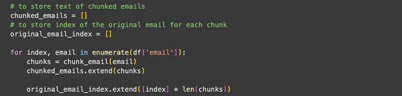
As in my previous posts, I first chunk the emails into smaller chunks. This is especially useful for fine-tuning because chunks from the same email can be assumed to be semantically related and used to create positive pairs.

Step 2: Create input pairs

Next, we generate the input pairs. To improve fine-tuning, I created a mix of easy and hard pairs:

Easy pairs (80%)
- Straightforward cases that allow the model to learn simple semantic similarity.
Hard pairs (20%)
- More challenging cases that help the model generalise better.
- These pairs are tricky since they may appear similar but are actually different (hard negative), or appear different but are actually similar (hard positive).

Initially, I started with only easy positive and negative pairs, but I realised that including hard pairs is needed for the embedding model to generalise better.

Positive Pairs

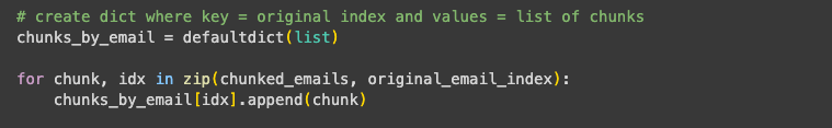
For easy positives, I iterated over chunks_by_email, a dictionary with the original email index as the key and a list of chunks as the value.

Only emails with at least 2 chunks were considered, This is since a minimum of two different chunks from the same email are needed make a pair.

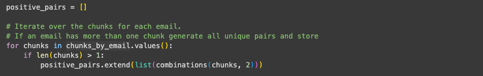
I used Python’s combinations to generate all possible pairings of chunks for that email.

For example:

Email 1: chunk a, chunk b, chunk c

Positive pairs for Email 1: (chunk a, chunk b), (chunk a, chunk c), (chunk b, chunk c)

All positive pairs are stored in a list, ready for processing.

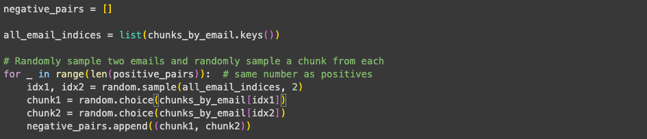
Negative Pairs

For easy negatives, I:

Randomly sampled two different emails.
Selected a random chunk from each email to form a negative pair.
Repeated this process until the number of negative pairs equalled the number of positive pairs, ensuring a balanced dataset.

Hard Pairs

Before diving into the implementation, I thought it would be useful to explain concept of hard pairs, as they can be tricky to understand:

Hard positives: Pairs that initially seem different but are actually similar in meaning.
Hard negatives: Pairs that look similar on the surface but are actually unrelated.

To save time, hard pairs were created for both positive and negative cases simultaneously.

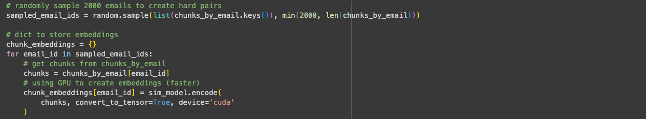
I first generated embeddings for 2,000 emails, (~20% of the dataset) and then iterated over pairs of different emails from this sample. The reason for this is that comparing chunks within the same email usually produces trivial pairs, whereas comparing chunks across emails creates more challenging pairs.

For each email, I generate embeddings using the same Sentence Transformer model that I later use for fine-tuning. With these embeddings, I constructed a similarity matrix between all chunks in one email and all chunks in the other email, using the cos_sim method from the sentence_transformers package.

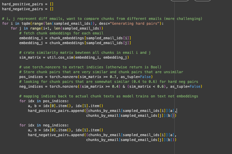
Based on this similarity matrix, I used thresholds to select hard positive and negative pairs:

Hard positives: similarity ≥ 0.7. These are chunks that are clearly related in meaning but not identical, making them useful for training the model to recognise semantic similarity.
Hard negatives: similarity >= 0.4 and <= 0.6. These are pairs that appear somewhat similar but actually come from different contexts, making them distractors for the model.

This way, the model is trained not only on obvious examples but also on ambiguous cases which provides a more realistic training set.

I think this concept would work even better if the emails were organised into threads, However, since the Enron dataset is not threaded, we can only assume that chunks from the same email are semantically similar.

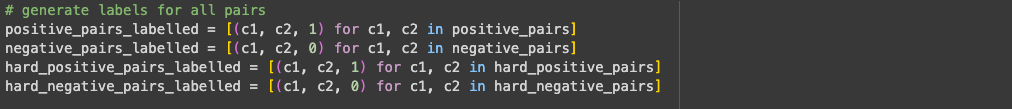
Step 3: Add labels and Set Aside Hard Pair Test Set

Assign a label of 1 for positive pairs and 0 for negative pairs.

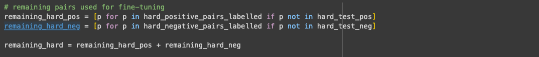
I then set aside a small test set of hard pairs to evaluate the model on challenging cases. This test set includes 200 hard positive pairs and 200 hard negative pairs.

The remaining pairs were used for fine-tuning:

I thought doing this would let me assess how well the model performs on known difficult examples and give a realistic measure of its performance.

Step 4: Combine positive and negative pairs

Concatenate all positive and negative pairs into a single list, then shuffle it.

Shuffling prevents the model from seeing all positive or all negative pairs consecutively, which reduces bias and stabilises training.

Step 5: Prepare Data for Fine-Tuning

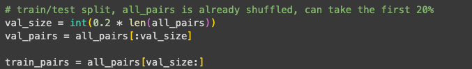
First, I split the data into train/test sets: 80% for fine-tuning, 20% for testing.

Next, I formatted the training data for the Sentence Transformer model:

Input pairs should be of type InputExample.

Wrap the data in a DataLoader and create batches for faster training. Processing batches instead of single pairs stabilises learning and prevents the model from overreacting to unusual examples.

I also created an evaluator using EmbeddingSimilarityEvaluator, which assesses performance after each epoch.

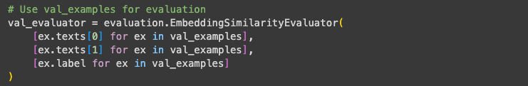
It calculates metrics such as Pearson and Spearman correlation between the predicted similarities and the ground truth labels (1/0). This let me to track whether the model improved across epochs.

Step 6: Train

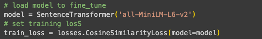
I decided to use the smaller model as the dataset (~10,000 emails) was too small for a larger transformers and risk of overfitting would be higher.

I also used CosineSimilarityLoss as the training loss function, which measures the similarity between embeddings of positive and negative pairs.

The model was fine-tuned for 3 epochs, giving a training size of ~30,000 rows. Below, are some of the params I set:

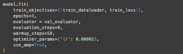
Below, are some of the params I set:

train_objectives=[(train_dataloader, train_loss)]

Defines what the model will train on.
train_dataloader contains the input pairs.
train_loss is the loss function used to update the model weights

epochs=3

Number of times the model will iterate over the entire training dataset.

evaluator = val_evaluator

Defines evaluation method to use during training.

evaluation_steps=0

Set to 0 so evaluation is performed at the end of each epoch.

warmup_steps=50

The number of steps at the start of training where the learning rate gradually increases from 0 to the set value (below)
Helps prevent sudden large updates at the beginning and so stabilises learning.

optimizer_params={'lr': 0.00002}

lr is the learning rate, controlling how large each weight update is.
0.00002 is small learning rate, I didn’t want to take too much away from what the model has learnt already.

use_amp=True

Added to speed up training, instead of using full float 32 uses float 16 to reduce memory usage for GPU.

Step 7: Quick Assessment of Results

During fine-tuning, I used validation pairs to check how well the model was performing. I thought to use this as a guide if I needed to adjust training params.

Step	Training Loss	Validation Pearson Cosine	Validation Spearman Cosine
10607	0.0113	0.9765	0.8644
21214	0.0071	0.9816	0.8647
31821	0.0053	0.9832	0.8649

Pearson similarity improved steadily, reaching 0.985, indicating the model learned to identify semantically similar emails.
Spearman similarity stayed around 0.865, showing ranking performance was already decent.

These results seemed almost too good to be true, which I realised was because the validation set consisted mostly of easy pairs (since only 20% of the dataset consists of hard pairs). To better evaluate generalisation, I set aside 200 hard positive and 200 hard negative pairs as a separate test set.

Using the fine-tuned model, I generated embeddings for each chunk in a pair and calculated cosine similarity. High similarity for hard positives and low similarity for hard negatives indicated the model correctly captured subtle semantic relationships.

Class	Precision	Recall	F1-score	Support
0 (hard negatives)	0.90	0.84	0.87	200
1 (hard positives)	0.85	0.91	0.88	200

Overall, the model performed strongly on the hard pair test set. Precision for hard negatives was slightly higher than for hard positives, but F1-scores were very similar for both pairs.

Note: Strong performance on hard pairs does not guarantee equally strong performance in a vector database. Vector search tests how well embeddings position all emails in vector space, which determines nearest-neighbour retrieval. Good results on hard pairs show the model learned subtle semantic cues but doesn’t necessarily imply high vector search performance.

Step 8: Create the Embeddings and Output

Finally, I used the fine-tuned model to generate embeddings for the labelled dataset and saved them for use in my Vector Database notebook. I then loaded these embeddings to recreate the vector database and evaluate their impact on search performance.

Let’s take a look at whether the fine-tuning of embeddings has had any impact on the quality of my vector database!

Results

After fine-tuning my model on ~10,000 Enron emails, I re-encoded the labelled dataset and re-ran evaluations on different FAISS index types.

The scores below represent the proportion of nearest neighbours that shared the same label:

Flat L2: 0.56
IVF: 0.54
HNSW: 0.56

Surprisingly, the fine-tuned embeddings performed slightly worse than the out-of-the-box Sentence Transformer embeddings. It could be that fine-tuning process may have actually overwritten some of the general knowledge the base model had learned during pretraining leading to some information loss.

Why Fine-Tuning Didn’t Improve Results

1). Hard Pairs

I created both positive and negative hard pairs so the model could learn from some challenging cases. However, these made up less than 20% of the dataset (with some reserved for testing).

While the model performed well on the test set of hard pairs, 10,000 emails likely wasn’t enough to influence how the model positions all vectors in the embedding space (which is needed for better retrieval).Even increasing the proportion of hard pairs from 20% to 50% would probably not have made much of difference.

2). Dataset size

Fine-tuning on ~10,000 emails is relatively small for a transformer model, even a smaller Sentence Transformer.

Expanding beyond 10,000 emails could improve results, as more data usually helps models generalise better. However, training was slow and I often ran into Colab GPU timeouts, which made increasing the dataset difficult.

Based on these factors, I decided not to continue iterating over the fine-tuning process and instead focus on building my web app. From the steps I’ve already taken and the impact they made, I expect any other changes would only come with slight improvements. At best, the fine-tuned embeddings might perform slightly better, but more likely it would remain on par with the out-of-the-box embeddings.

Summary

Next, I’ll focus on building the web app so users can try out similarity search themselves. I’ll use Docker to make the app easy to deploy and access. I also plan to reflect on the project, covering the challenges I faced and sharing the key lessons I learned along the way.