Email Genie: Modelling 🕺

In the Email Genie series so far, I began by cleaning up the messy email data, removing as much noise as possible. After that, I tried out different methods to vectorise the emails and found that Sentence Transformers gave the best results. Next, I manually labelled a subset of ~1,000 emails into five categories, based on recurring themes I noticed during my analysis. To know more about the labels, see this post.

Now comes the part I always look forward to the most… modelling! In this post, I’ll walk through the different classification models I experimented with, share how I implemented them and talk about some of the challenges I ran into along the way.

---

Classification Models

First, let’s talk about which models I decided to experiment with and why.

1) Logistic Regression

I always like to start with a simple model like Logistic Regression because it’s easy to train and quick to interpret. I find these kinds of models make a great baseline as they help set a benchmark for performance. If more complex models don’t perform better, that usually means there is an issue with the data - either there’s not enough of it or the data just doesn’t provide enough information for the model to learn well from it.

2). Support Vector Machine (SVM)

After looking at which models are best suited to high-dimensional data like embeddings, I came across SVM classification models. SVM is similar to other classifiers in that it tries to find the “best” way to separate the classes, but it takes things a step further. It’s specifically trained to find the largest gap between the classes and only focuses on the hardest cases in the dataset which are the ones closest to the class boundaries.

This means it doesn’t need thousands of examples to learn well. By learning from just those edge cases (called support vectors) it can understand the decision boundary for each class. So to me, this seemed like the perfect model to use on my limited, high-dimensional labelled data.

3). Random Forest

The last model I wanted to try was Random Forest. This model is quite different from the other two, as it’s an ensemble model. Essentially, Random Forest combines results of multiple decision trees to make a final prediction, this is known as bagging. In the future I will do a separate blog post introducing the different types of models!

I thought it would be interesting to try Random Forest to see if a non-linear model could capture patterns that the previous models might miss, especially if there were any patterns between features that weren’t captured by straight-line boundaries.

Implementation

Below I’ll walk through how I trained each model and compared their performance.

Step 1: Load Embeddings

I started by loading embeddings for my labelled dataset. To do this, I used a Sentence Transformer model to generate embeddings for all the emails. (If you want to know more about how embeddings work, I covered that in earlier Email Genie posts here).

Step 2: Encoded Labels

I decided to encode the labels by using LabelEncoder. This essentially transforms my categorical labels into numeric labels.

Step 3: Split X and y

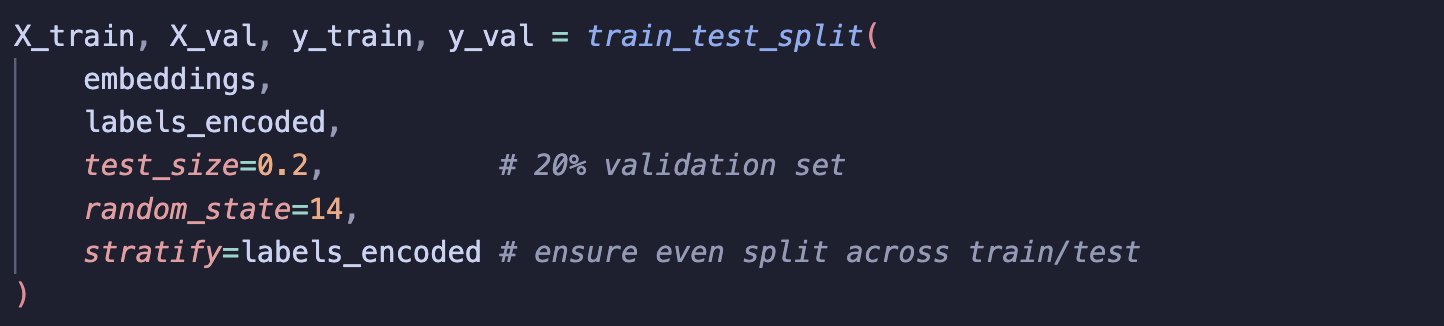
Split the data into X and y, and use stratify when creating training and validation sets to ensure the label distribution stays the same in both splits to help minimise bias.

Step 4: Define models to train

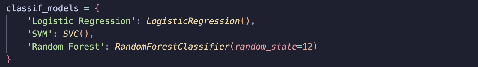
Rather than writing separate code blocks for each model, I defined all the models in a single dictionary making it easier to loop through and train.

Step 5: Train models and store results

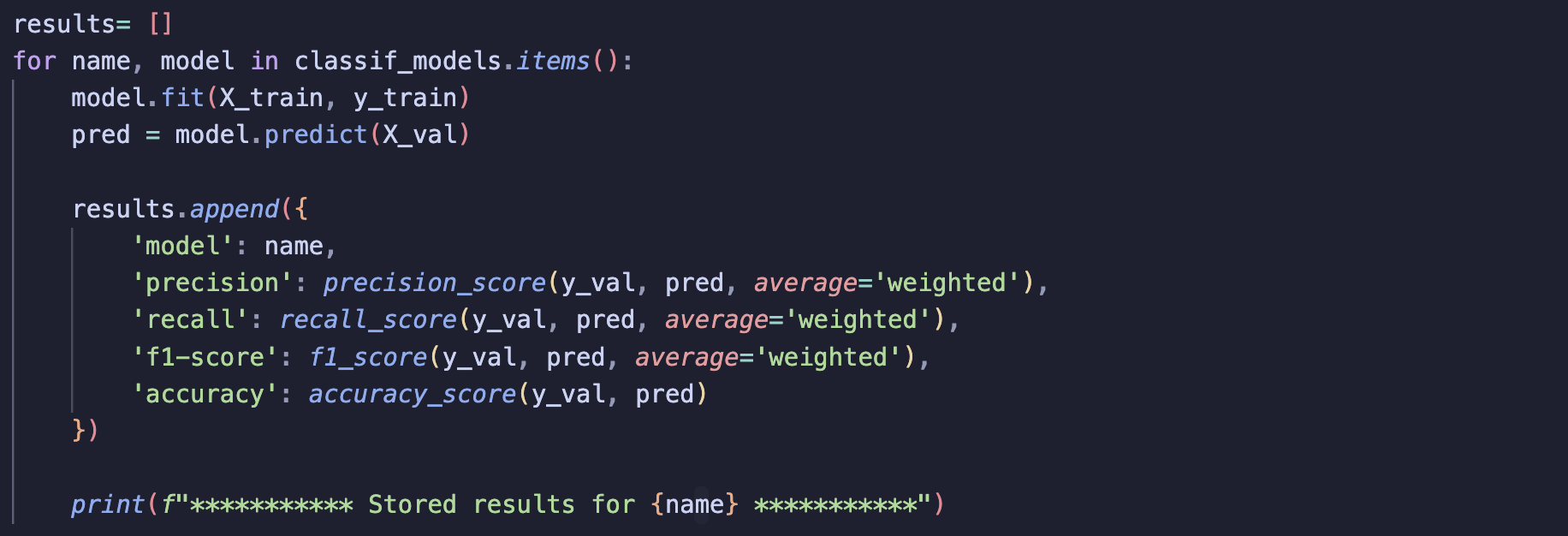
Finally, I trained each model in a loop, storing their predictions and metrics for comparison.

Results

Let’s take a look at how the three models did:

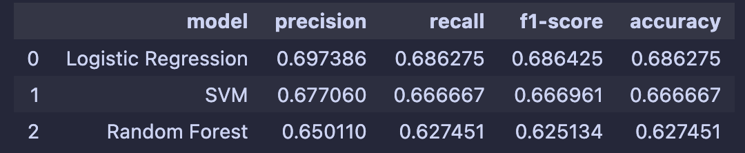
Performance across all three was similar, with Logistic Regression slightly outperforming the others. Using more complex models didn’t seem to offer any improvement in results. This suggests the issue is likely with the dataset, I think it may be too small for what I’m trying to do and the labels may not be reliable enough.

To be honest, I was quite eager to get the labelling done, and looking back, the quality may have suffered. For simplicity, I decided to classify each email with a single label. In hindsight, that might not have been the best decision as many emails could easily fall under multiple categories. I saw this overlap during the TF-IDF analysis and should have considered this more carefully.

Originally, I planned to do hyperparameter tuning on the best-performing model, but at this point I don’t think it would make much difference.

---

Fine Tuning DistilledBERT Classifier

For a while, I wasn’t too sure what the next step for this project should be. I wanted to avoid going back and manually labelling another 1,000 emails as it’s rather time-consuming and for me mentally draining…

So instead of expanding the dataset, I started thinking about how to make the most of the data I already had. That’s when I decided to try fine-tuning DistilBERT, not for generating embeddings, but for training it as a classifier.

Even though I only had around 1,000 labelled examples, I thought fine-tuning was still worth trying. DistilBERT already has a strong understanding of language, so I can fine-tune to guide it with the labels and let it learn specific patterns in my dataset.

How Fine-Tuning for Classification Works

In previous posts, I’ve explained BERT’s architecture and how it produces embeddings. DistilBERT follows the same process but with a more lightweight architecture like fewer layers, no poling, etc. It’s designed to be faster and perfect for cases where a GPU isn’t available.

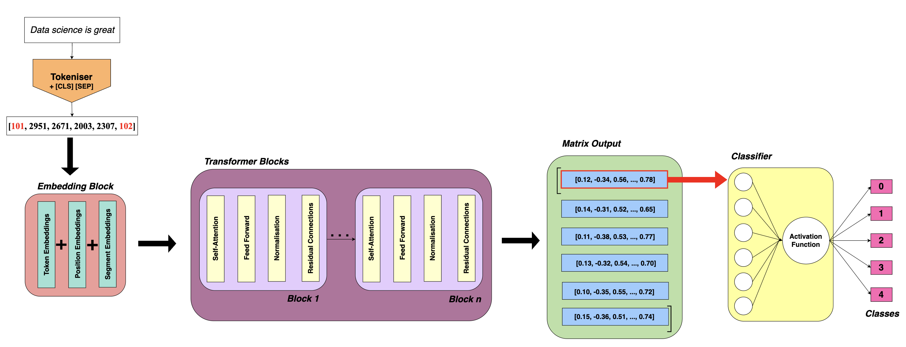
Below, I’ve expanded my previous BERT diagram to show the extra parts needed to turn BERT into a classifier.

Note: The process is the same for DistilBERT.

Following the output of the embedding matrix, a small neural network is added. Typically this is just a single fully connected layer followed by an activation function. As a reminder, some activation functions like softmax and sigmoid convert raw scores (logits) into probabilities. Since each email in my dataset has only one label, I use softmax, which is also the default in the DistilBertForSequenceClassification model.

Inside the embedding and transformer blocks of DistilBERT are weights that have already been pre-trained on millions of text examples. By default, when using DistilBERT as a classifier, all of these weights are updated during training and the entire model is fine-tuned on the new data. However, since my labelled dataset is relatively small, I chose to freeze a large portion of the model’s weights and only update the weights in the last few layers. This helps reduce the chance of overfitting while allowing the model to adapt to the data.

During fine-tuning, the embedding for the [CLS] token is updated so that it acts like a summary of the input text. This updated [CLS] embedding is the only one passed to the classifier layer. Previously, this [CLS] token indicates the start of an embedding and does not provide a summary. By only passing the CLS embedding, the classifier can be fairly simple (single dense layer).

Implementation

Step 1: Separate out the emails and labels

As with training the classifier models before, I start by separating the emails and their labels. I also encode the labels.

Step 2: Split X and y

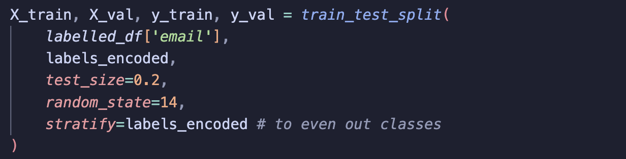
Next, I split the dataset into training and validation sets using a stratified split. Stratifying by labels ensures that the distribution of labels remains balanced across both training and validation data. This helps the model learn better and minimises bias.

Step 3: Tokenise the emails

Similar to when creating embeddings, I tokenise the emails using the same tokenise_and_chunk function from previous posts.

Like before, I chunked the emails since most exceed the 512-token limit of DistilBERT:

a) Training Set

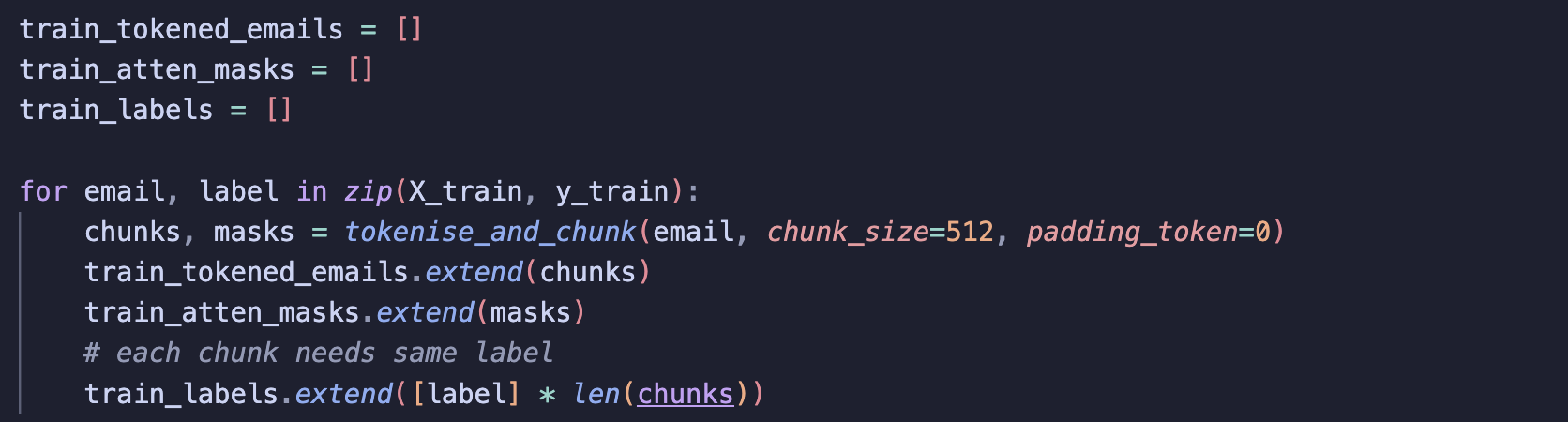
Here, I loop over each email and its label, pass the text through my function, and collect all the chunks and attention masks. I had to be careful here to be sure all chunks from the same email also shared the same label!

b) Validation Set

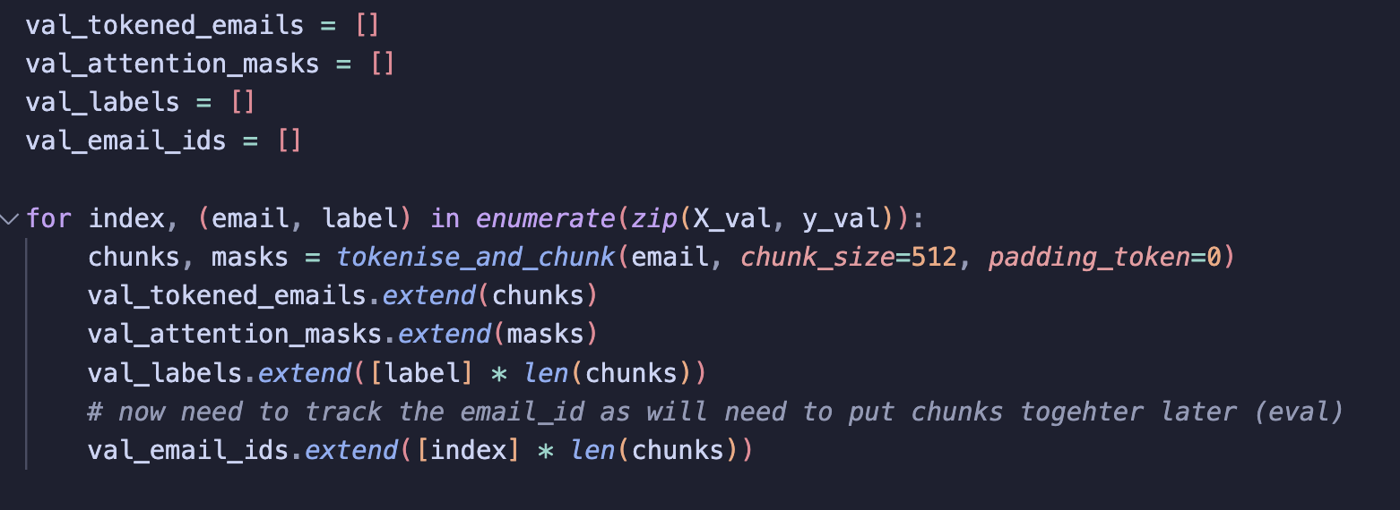
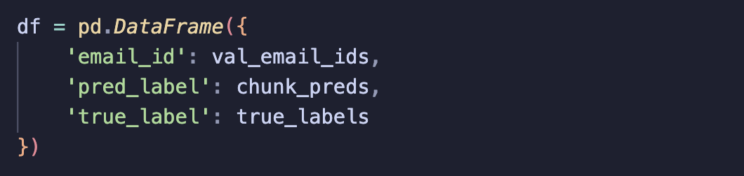
For the validation set, I use the same approach but here, I also store an email_id for each chunk. This is because the model will make a single prediction for each chunk (since long emails are split).

At first, my evaluation results looked rather low with most metrics under 50% and I realised this was because I was using trainer.evaluate() to calculate metrics. Usually this works well, but the Trainer does not know that emails have been chunked and so compares each chunk’s prediction against the original email-level label. This can cause issues because each chunk is only part of the email, and in some cases information that determines the category may be in later chunks. This means the model’s predictions for a single chunk can be incorrect causing the low metrics.

To get a true sense of how well the model performs, I needed to group all the chunks that have the same email_id before evaluating the model!

Step 4: Build Datasets

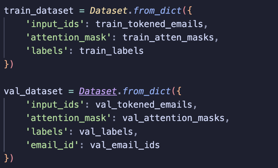
The classifier requires data as a Dataset object. Using the Hugging Face documentation, I created Dataset objects for the training and validation sets.

Step 5: Define model and training args

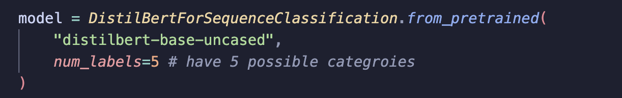
I defined the classification model (a DistilBERT with an added classification layer on top) and set the training arguments.

The TrainingArguments define how training should run for example how big each batch should be and how many epochs to train for. Here are the arguments I set:

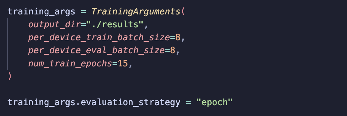
• output_dir: Directory to store the trained model

• per_device_train_batch_size: Number of samples in each training batch

• per_device_eval_batch_size: Number of samples in each evaluation batch

• num_train_epochs: Number of times to iterate over the entire training dataset. I set this to 15 since I have a small dataset and wanted to give the model more opportunity to learn patterns.

• evaluation_strategy: Defines when to evaluate the model I chose to evaluate at the end of every epoch to monitor performance and spot overfitting.

I also then needed to define a Trainer object. This basically handles the whole training and evaluation loop by feeding batched data into the model, running forward and backward passes, updating weights, etc… Here are the parameters I set:

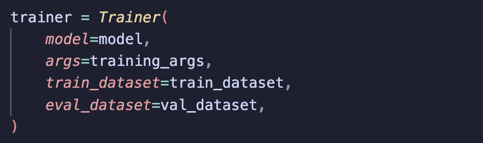
• model: The model to fine-tune

• args: The training arguments described above

• train_dataset: The dataset used for training

• eval_dataset: The dataset used for evaluation

Step 6: Freeze weights

As discussed earlier, I chose to partially freeze DistilBERT’s weights to help minmise the risk of overfitting on my small dataset. Since the [CLS] embedding is updated during fine-tuning, we need to make sure this part remains unfrozen. By freezing/unfreezing, I mean allowing the weights to be updated during training or keeping them fixed.

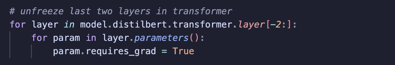
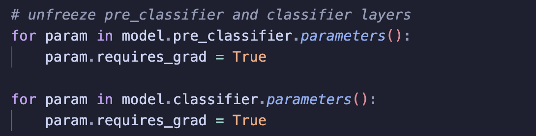
If we look at the diagram, we can see that the [CLS] embedding is updated in the transformer block, this means the last few layers must be unfrozen to allow the embedding for CLS to be updated. Of course, the classification layer on top must also be unfrozen and trainable. So, I froze all layers and only allowed the weights in the last few layers to update during training.

Step 7: Train the model

With everything set up, it’s time to train the model! To do this, I called the Trainer object and used .train().

This step took a fair while to run!

Step 8: Assess results

Since I chunked my emails, I had to evaluate my results manually.

a) Run .predict

This outputs predictions as an array of logits for each chunk, along with label_ids which are the ground-truth labels.

b) Extract predictions

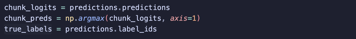
From the logits, I convert each chunk’s output into a predicted label and also extract the true label for each chunk.

c) Collate predictions for each chunk

Since each email is split into multiple chunks, I group the chunk predictions by email_id and combine them into a single email-level prediction using majority voting.

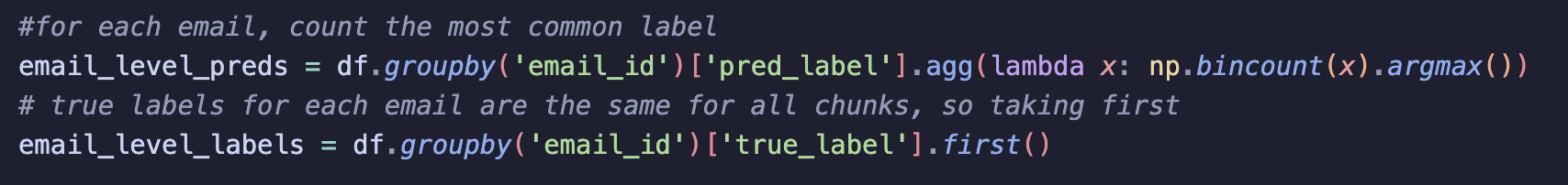
agg function does majority voting by:

• np.bincount(x): counts how many times each predicted label appears among the chunks of that email.

• .argmax(): selects the label with the highest count

For true labels, since all chunks of the same email share the same true label, I do .first()

d) Calculate metrics email level

• Pass in email level predictions and labels to the classification metrics

• Results look more realistic, let’s take a closer look …

Results

Accuracy	Precision	Recall	F1-Score
67.7	68.2	67.7	67.7

Overall, DistilBERT, even with fine-tuning, is not really outperforming the simpler classification models I tested. This confirmed my initial concern: there simply isn’t enough labelled data for any model to learn effectively. Since I’m not planning to spend time labelling more data, I may need to reconsider the scope of the project to better suit the data I have.

---

Summary

Classifying a sample of emails from the Enron dataset proved to be quite challenging. I wasn’t expecting great performance since email text is very noisy, but I did hope that different classification models would improve on the logistic regression baseline. This wasn’t really seen, I think the main reason for this was the dataset. It wasn’t large enough for the models to learn well enough, especially with text as nuanced as emails.

Instead of spending more weekends labelling more data, I’ve decided to slightly change the project scope. I’m now thinking to explore semantic similarity using vector databases. I’m not sure yet how well this will perform, but I’m excited to try it out and learn more about vector databases!